Image Processor
Filters & Warps
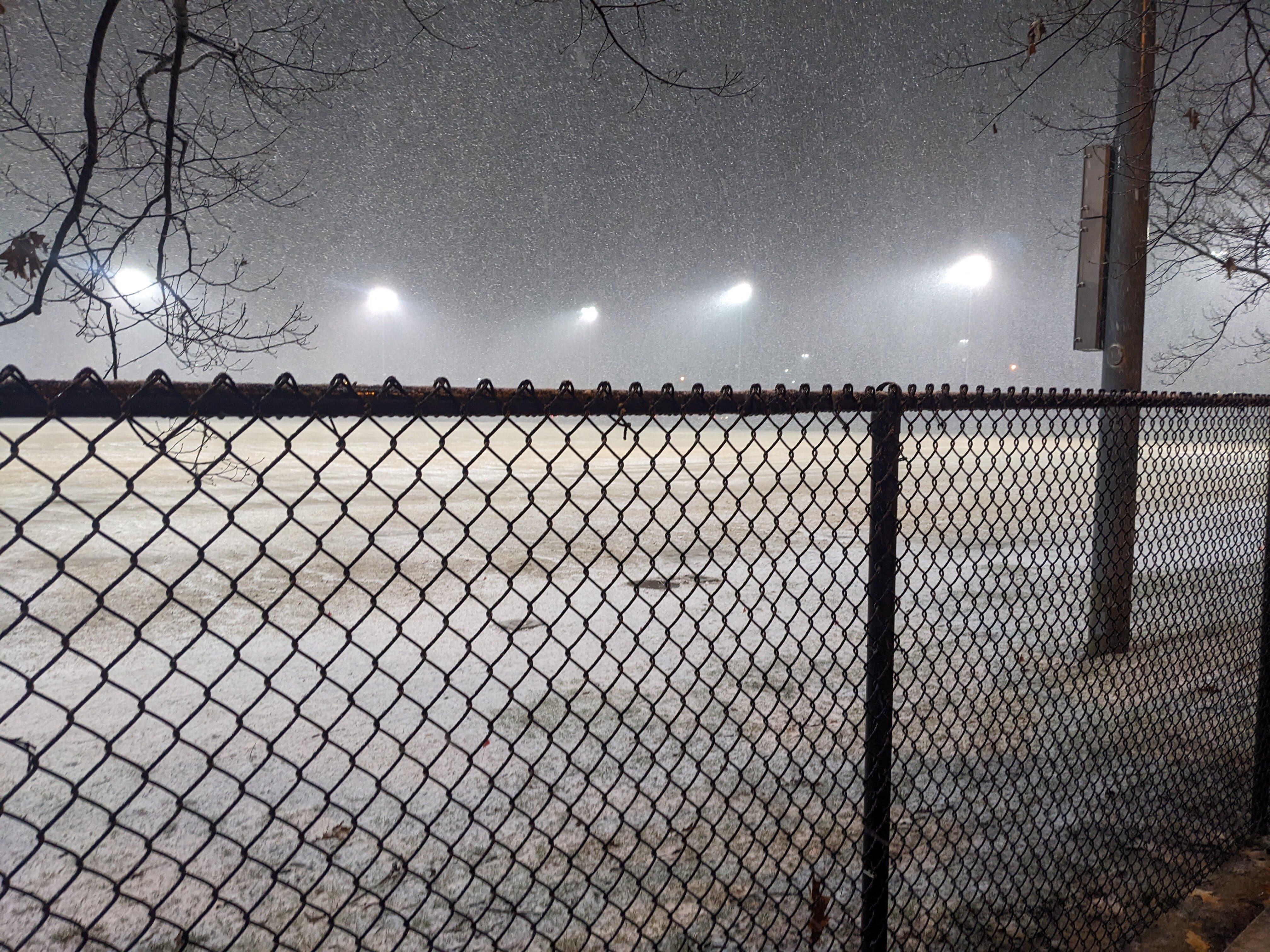
“Traditional” image processing techniques can be separated into two broad categories, filters and warps. Filters are image manipulations which alter pixel color, whereas warps alter pixel positions. Filters, warps, their combinations, and machine learning are largely the difference between a modern phone’s 12MP photo, and a 12MP photo taken on a 5-6 year old phone.
I won’t be going over machine learning techniques in this article, but if it wasn’t already evident by the bombardment of tech ads and the news, machine learning is at the cutting edge of image processing.
This article is dedicated to explaining a variety of artistic and practical image filters and warps, all of which I’ve implemented to better understand image processing. For both filters and warps I've listed them in order of ascending complexity and required knowledge, but none are so complex as to require coming in with a high technical background.
I've included pseudocode with all of my explanations, but you can also find all my c++ implementations on Github
Representing Images
Before getting into the nitty-gritty of image transformations you need to understand how images are represented.
Color
Images are represented as a grid of tiny squares called pixels, (crazy I know) which make up images. For grayscale images each pixel has one "channel" value, which represents the brightness of the pixel. For color images each pixel has three channel's: red, green, and blue (in that order). These channels when combined together form the color of the pixels you see on your screen.
All channels of an image share the same valid range of values, however that range can be different depending on the image. Typically a bit-depth of 8 is used, which means each channel is in the range: \([0, 2^8-1]=[0, 255]\). Now this may not sound like a lot, but as the color of a pixel is the combination of its channels, the number of color combinations is: \(256^3 = 16,777,216\) colors, for each pixel.
Representing the Pixel Grid
If you've ever worked with 2-D data before then you know the standard representation uses an array of array's. This method does work for images, however it is typically not done for efficiency purposes.
The array's we represent an image with must be dynamic, as we want to have the ability to change the image in any way we want. However this poses a problem with the array of array's approach, as we can no longer guarantee contiguous memory our caching performance will suffer.
Generally we don't have to deal with matrices large enough for us to care, however images can require an incredible amount of elements to represent. For example my phone takes pictures with a resolution of 4080 by 3072. This means I need \(4080 \cdot 3072 \cdot 3 = 37,601,280\) indices (the times three is because of the three color channels).
As such we use a single dynamic array to represent the pixel data, and then manually map the (row, column) positions to the correct indicies. Luckily it's fairly easy to calculate this: given a row and column position, the correct pixel index is \((width_{image} \cdot row + col) \cdot |channels|\). For a grayscale image this will give you the one brightness value, for color this calculates the position of the red value. This means for color images to get the green and blue values as well, you need to add 1 and 2 respectively to the computed index.
With all that being said, for simple transformations where per-pixel values are determined independently of all other pixels, we don't even need to muck-about with the index calculation. Instead we can simply iterate over the image with a step equal to the number of color channels.
Table of Contents
Filters
Color Inversion
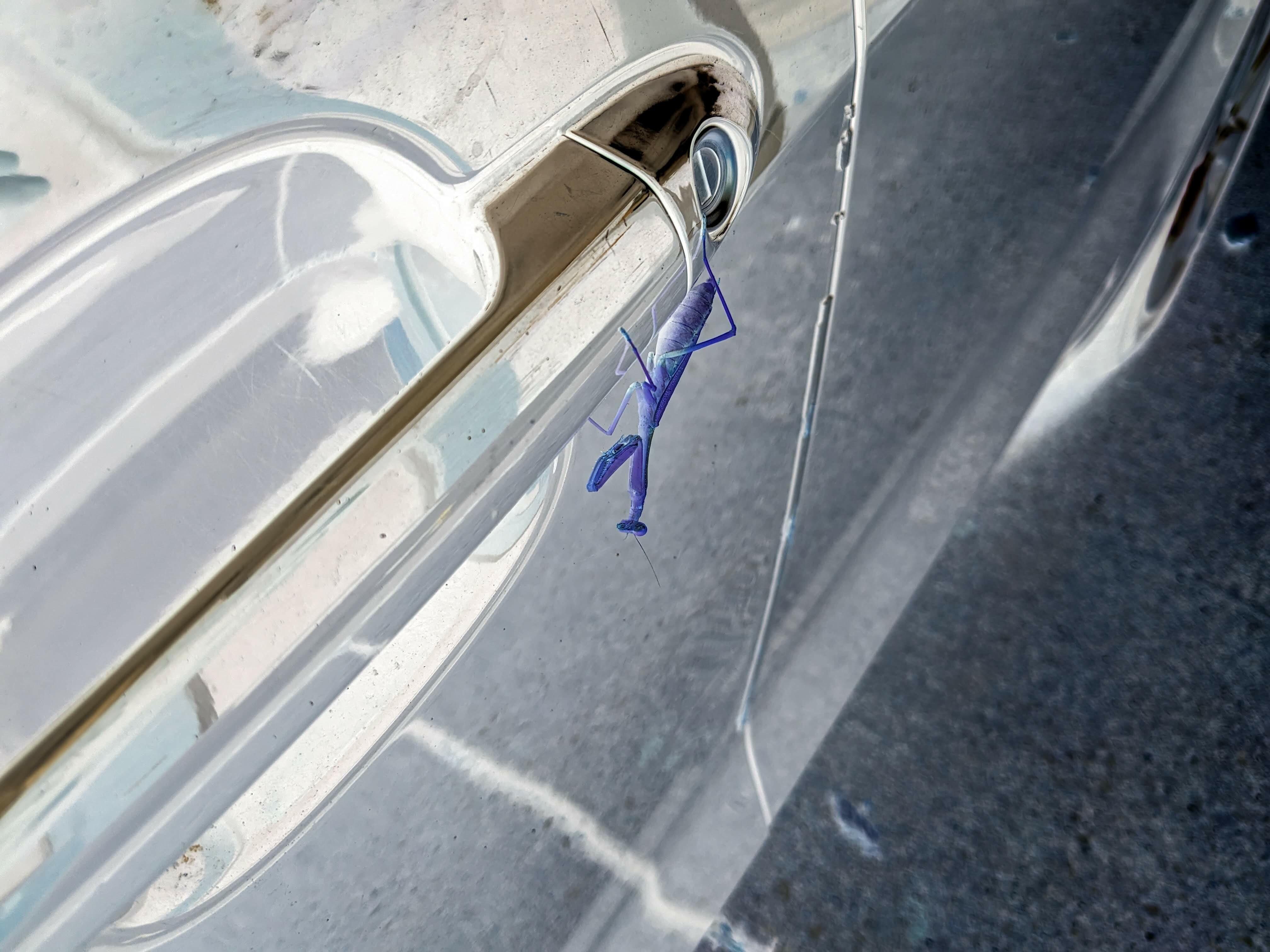
One of the simplest, if not the simplest image filter. To invert the color channels all you have to do is subtract each channel by the max color value.
To understand why this works you can think about the numberline; the opposite of -2 is 2, for -1 it's 1, and 0 goes to 0. This is exactly what we're doing for each channel, but now the range is [0, max_color]. So assuming 8-bit color, the opposite of 0 is 255, 1 is 254, etc.
You can also geometrically think about a 1-dimensional inverse as simply being the reflection over its midpoint.
  FUNCTION invert_colors()
    FOR i TO img_data_length STEP num_channels
        img_data[i] := max_color - img_data[i];

        IF num_channels = 3 THEN
            img_data[i] := max_color - img_data[i + 1];
            img_data[i] := max_color - img_data[i + 2];
        END IF
    END FOR

  END FUNCTION
Grayscale
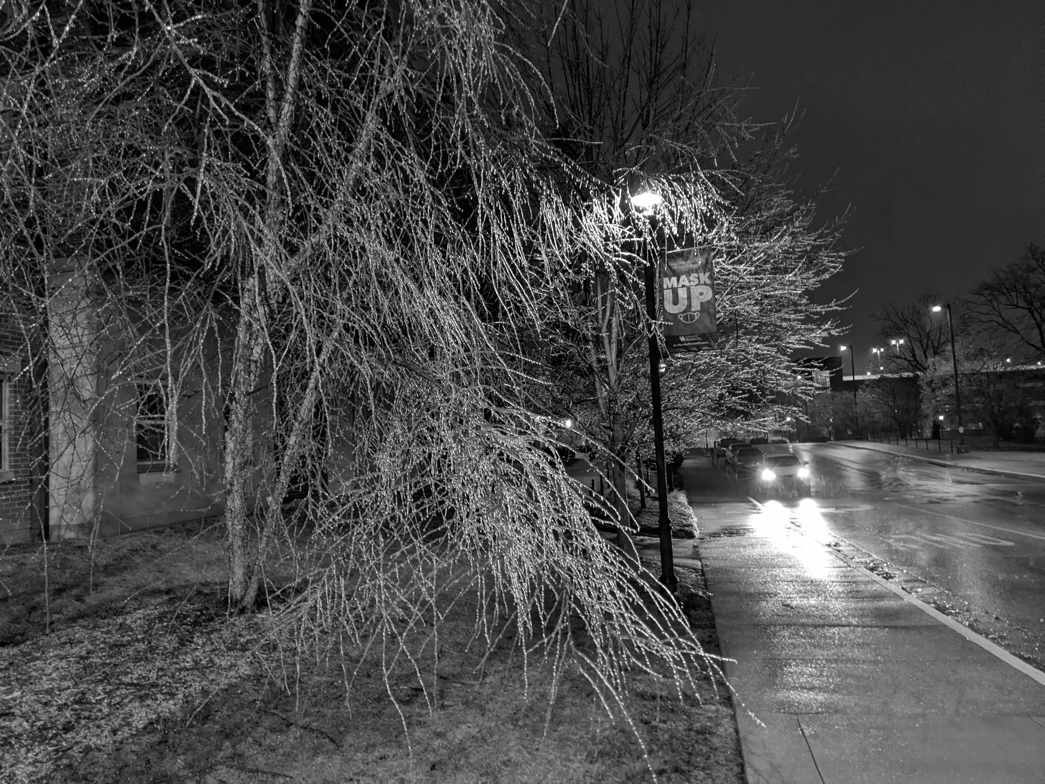
Grayscale does exactly what it sounds like, it takes all three color channels for a pixel and combines them into one gray channel. The simplest way to do this is to simply set the pixel as the average of its color channels.
The issue with this is that humans perceive the brightness of red, green, and blue differently. As such a more accurate way to grayscale an image is a weighted average which takes this into account. There are two standards for this, REC 709 and REC 601. REC 709 is the modern standard, and used for displaying HD content, whereas 601 is for older SD content.
*Note if you don't wish to switch to a grayscale image format, you can simply set each color channel to the computed gray value.
  FUNCTION grayscale()
    new_img_data := ARRAY OF (img_width * img_height)

    // weights determined by REC 709
    magic_weight_r := 0.2126
    magic_weight_g := 0.7152
    magic_weight_b := 0.0722

    // num_channels should be 3
    FOR i TO img_data_length STEP num_channels
      gray := img_data[i] * magic_weight_r + img_data[i + 1] * magic_weight_g + img_data[i + 2] * magic_weight_b

      // always divisible by num_channels, as STEP = num_channels
      new_img_data[i / num_channels] := gray
    END FOR
    img_data := new_img_data

  END FUNCTION
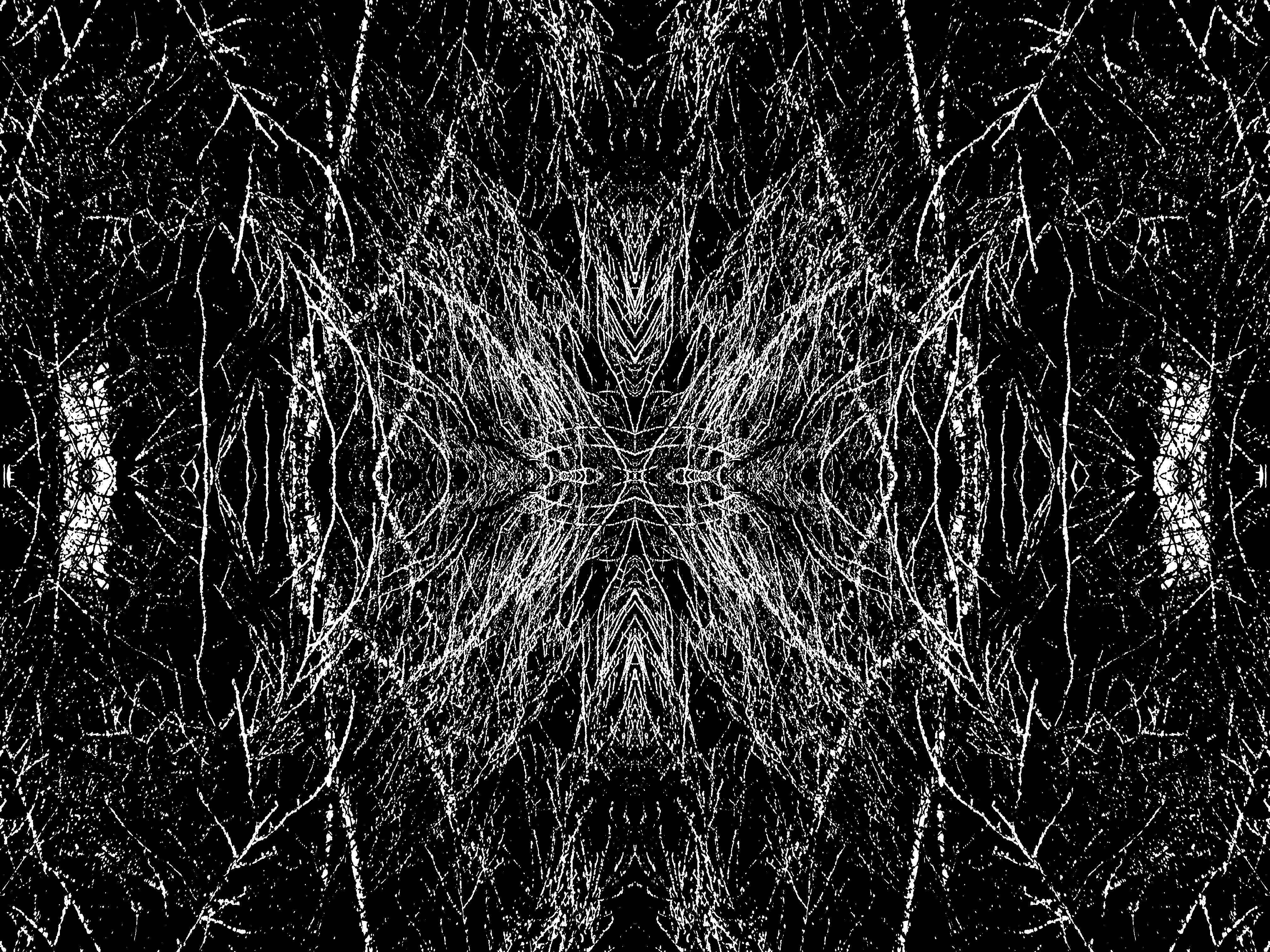
Thresholding
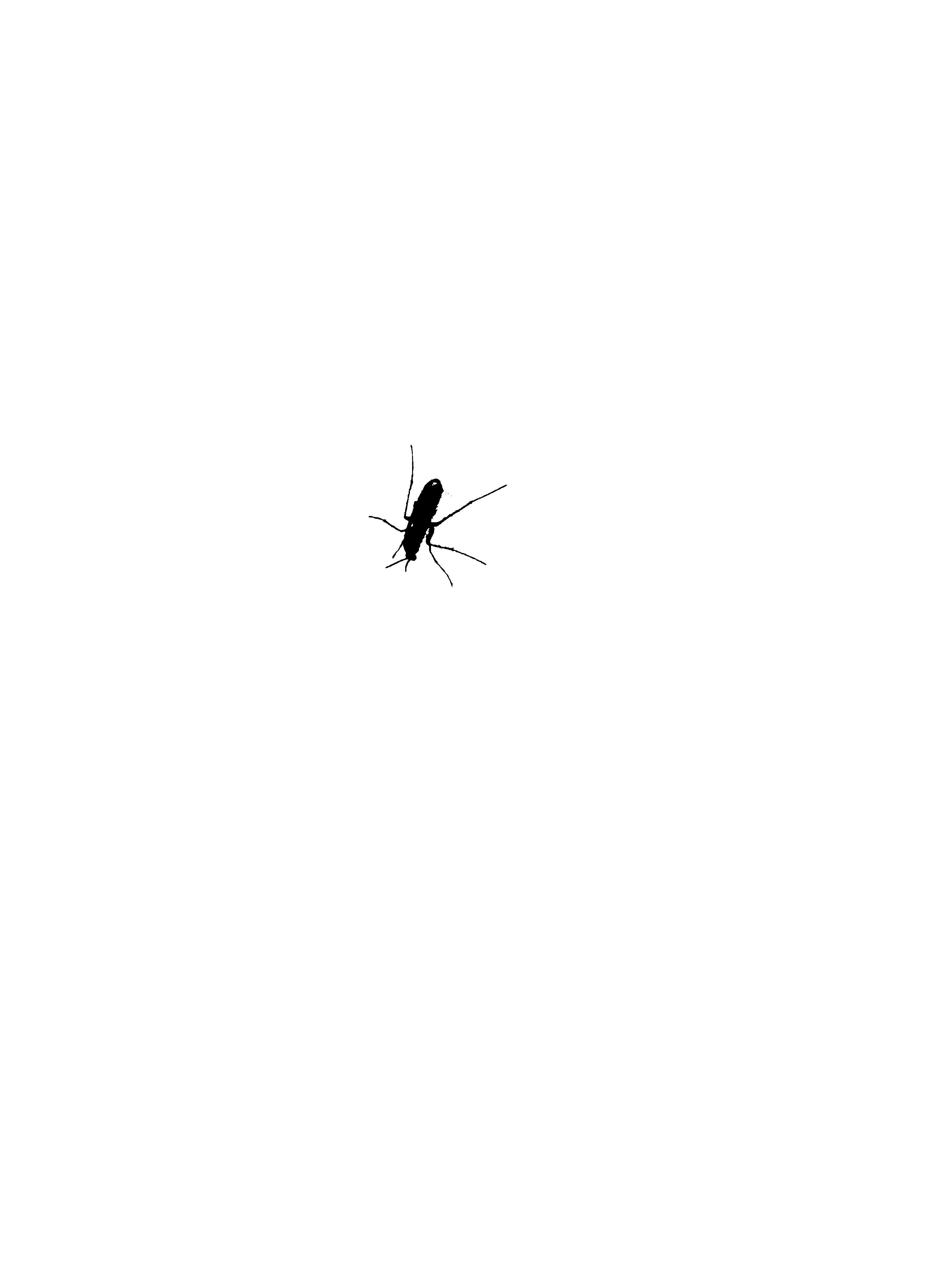
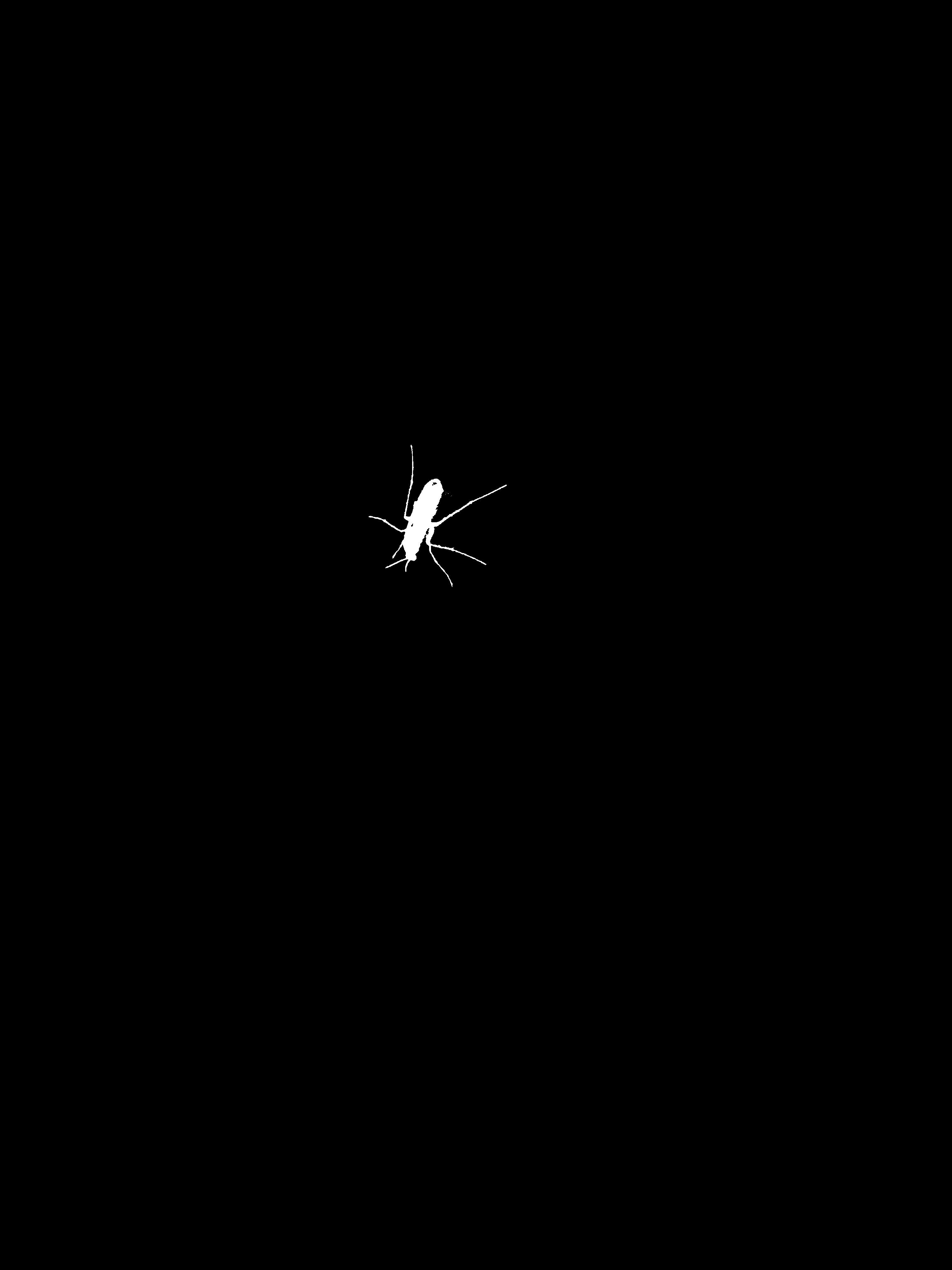
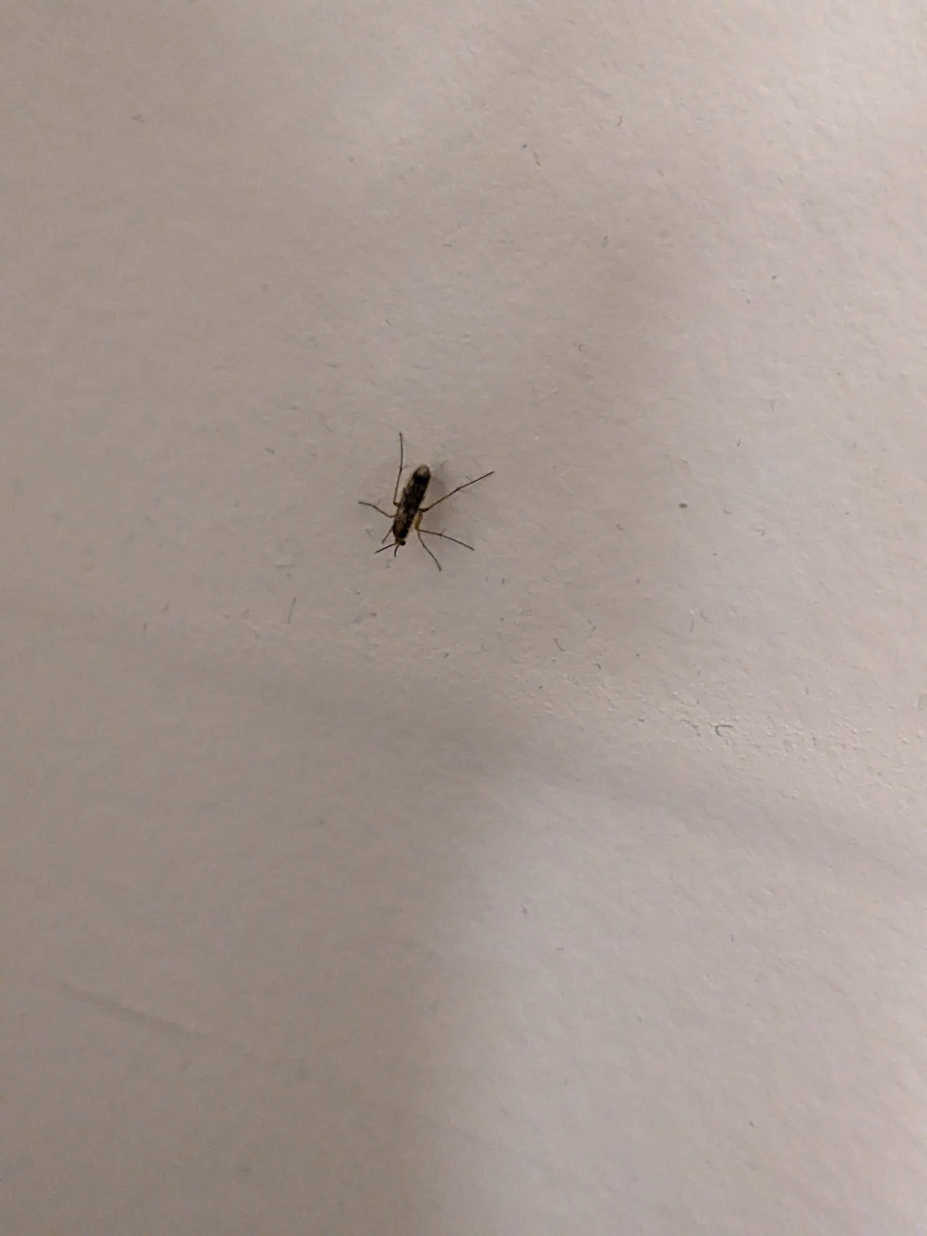
Thresholding is the most basic form of image segmentation. The purpose of segmentation is to programmatically separate out different parts of an image. This is very useful for visual analysis, and targeting specific area's to apply image filters and/or warps.
Thresholding works by taking some threshold value epsilon, and setting all pixels greater than epsilon to the max color value, and the rest 0.
It is also common to swap the black and white case's, as depending on the image a white subject on a black background may be preferable to a black subject on a white background.
  // assumes image is grayscale
  FUNCTION threshold(epsilon)

    FOR i TO img_data_length STEP num_channels
      IF data[i] > epsilon
        data[i] := max_color
      END IF
      ELSE
        data[i] := 0
      END ELSE
    END FOR

  END FUNCTION
Tint
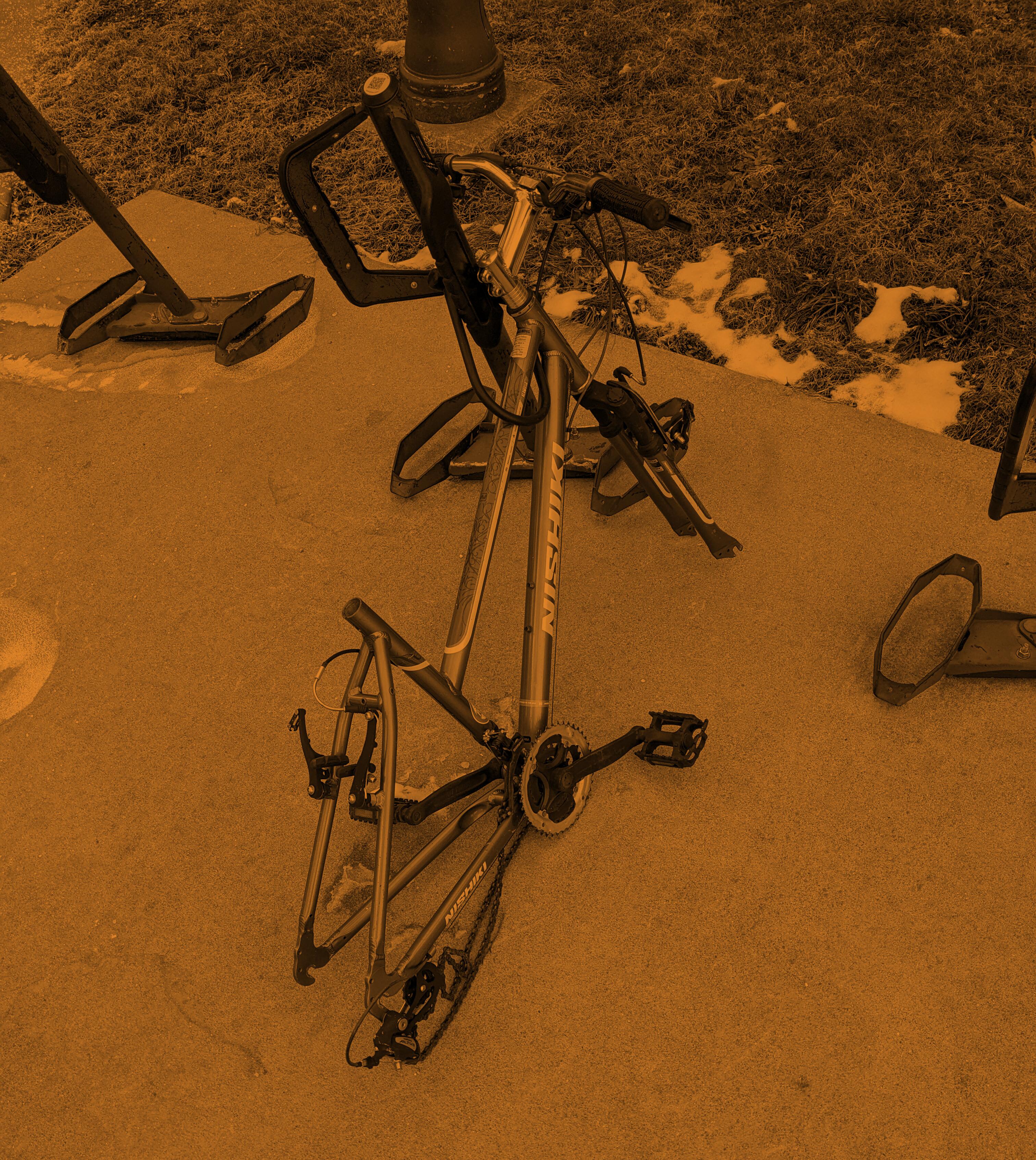
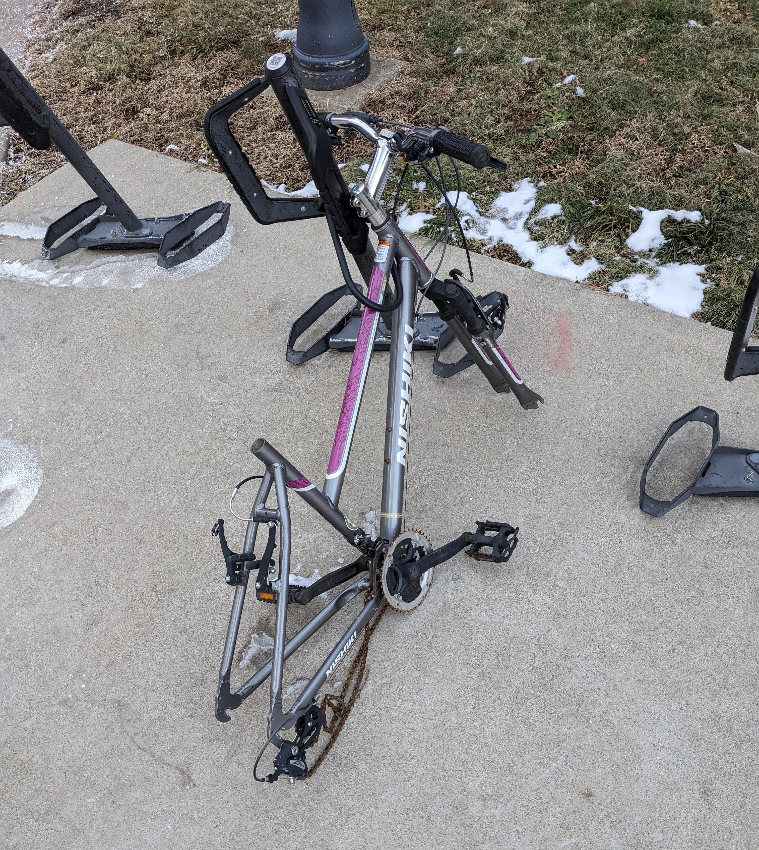
Tinting is just as it sounds, making an image appear as if it were tinted by a dye. This is mainly done for artistic purposes, and is pretty straightforward process:
- Get the (r, g, b) values of the wanted tint color
- Normalize the tint channels, i.e. divide each channel by the max possible color value
- Multiply each pixel channel by their respective tint channel
- (optional) If the output image is dark, multiply each channel by some constant > 1, to brighten up the image. However you must then also ensure the color value is not greater than the max.
  FUNCTION tint(r, g, b, brighten:=1)

    // normalize channels
    r := r / max_color
    g := g / max_color
    b := b / max_color

    FOR i TO img_data_length STEP num_channels
      data[i] := data[i] * r * brighten
      data[i + 1] := data[i + 1] * g * brighten
      data[i + 2] := data[i + 2] * b * brighten

      // if any color channel not in [0, max_color], clips to fit
      clip_pixel(i)
    END FOR

  END FUNCTION
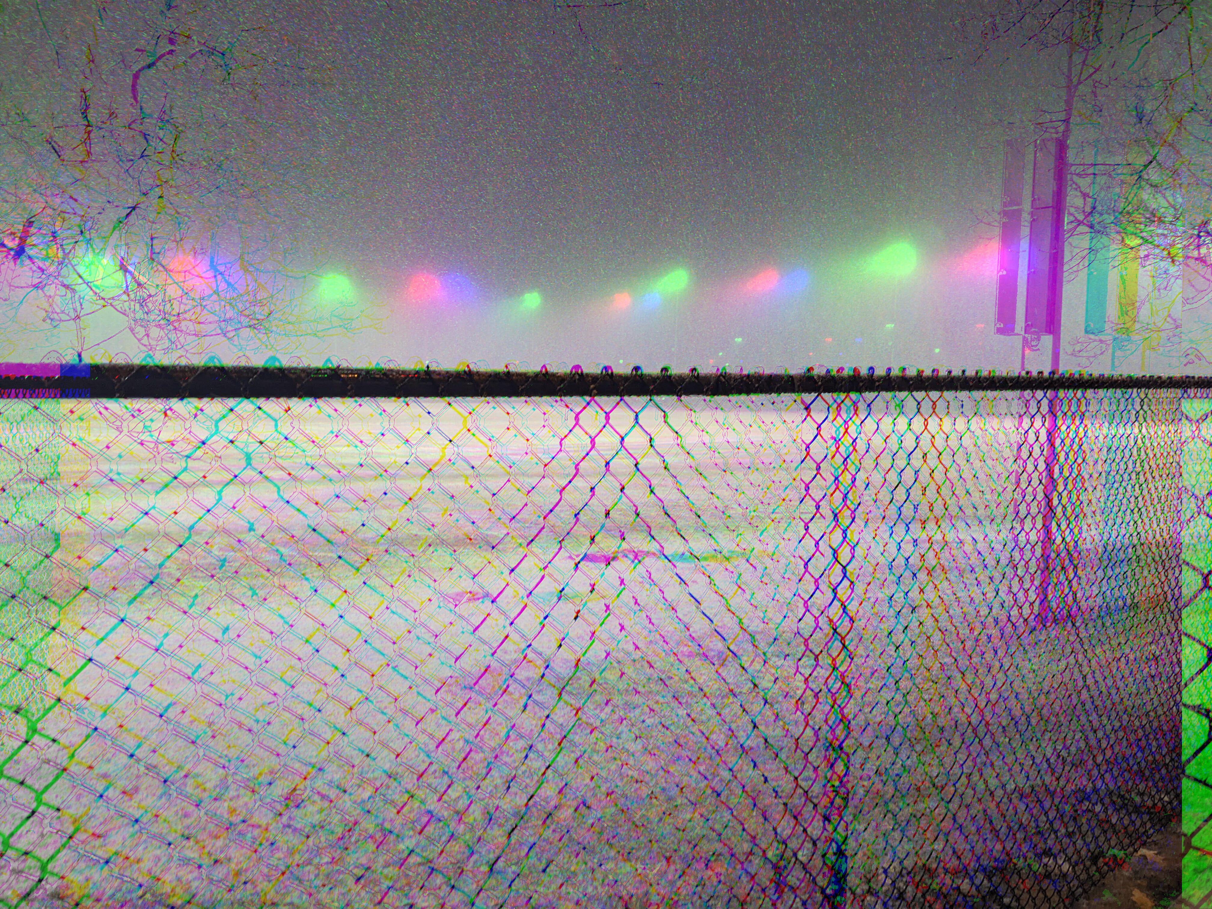
Chroma Shift
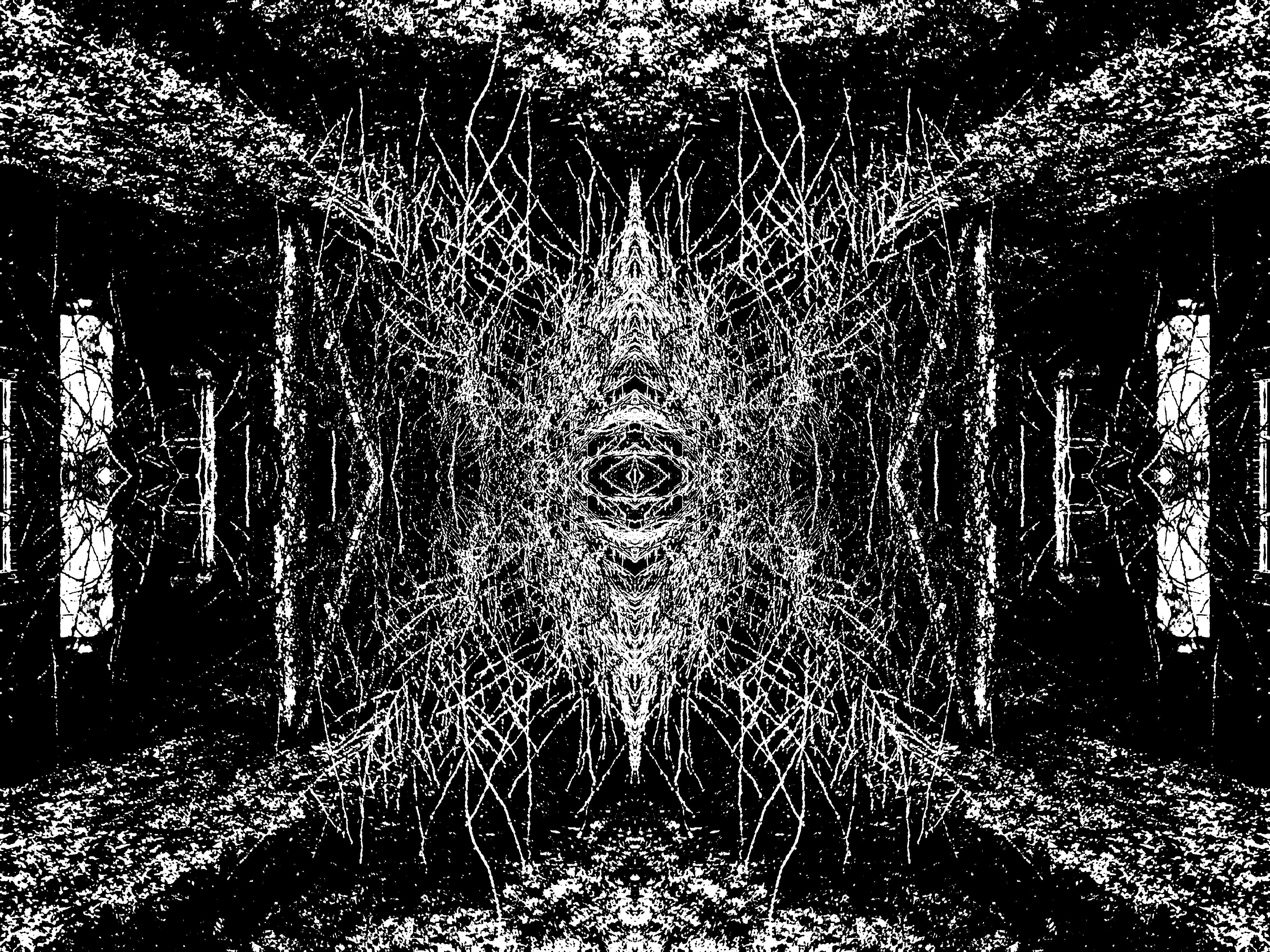
A chroma shift is done by taking the color channels of all pixels and shifting them left or right by some amount. This creates a “glitchy” effect as the color channels are now misaligned. This algorithm can also use thresholding to great effect, as it allows you to shift only selected parts of the image.
*Note this algorithm should not be done in-place, as that causes you to calculate shifts based on previously shifted channels.
  FUNCTION chroma_shift(r_shift, g_shift, b_shift)
    new_img_data := img_data

    r_shift := r_shift * num_channels
    g_shift := g_shift * num_channels
    b_shift := b_shift * num_channels

    FOR row TO img_height
      FOR col TO img_width
        pix_index := (width * row + col) * num_channels

        // conditionals prevent out-of-bounds indexing
        IF pixIndex + r_shift > 0 && pix_index + r_shift < img_data_length
          new_img_data[pix_index + r_shift] := img_data[pix_index]
        END IF

        IF pix_index + g_shift > 0 && pix_index + g_shift < img_data_length
          new_img_data[pix_index + g_shift + 1] := img_data[pix_index + 1]
        END IF

        IF pix_index + b_shift > 0 && pix_index + b_shift < img_data_length
          new_img_data[i + b_shift + 2] := img_data[pix_index + 2]
        END IF
      END FOR
    END FOR

    img_data = new_img_data

  END FUNCTION
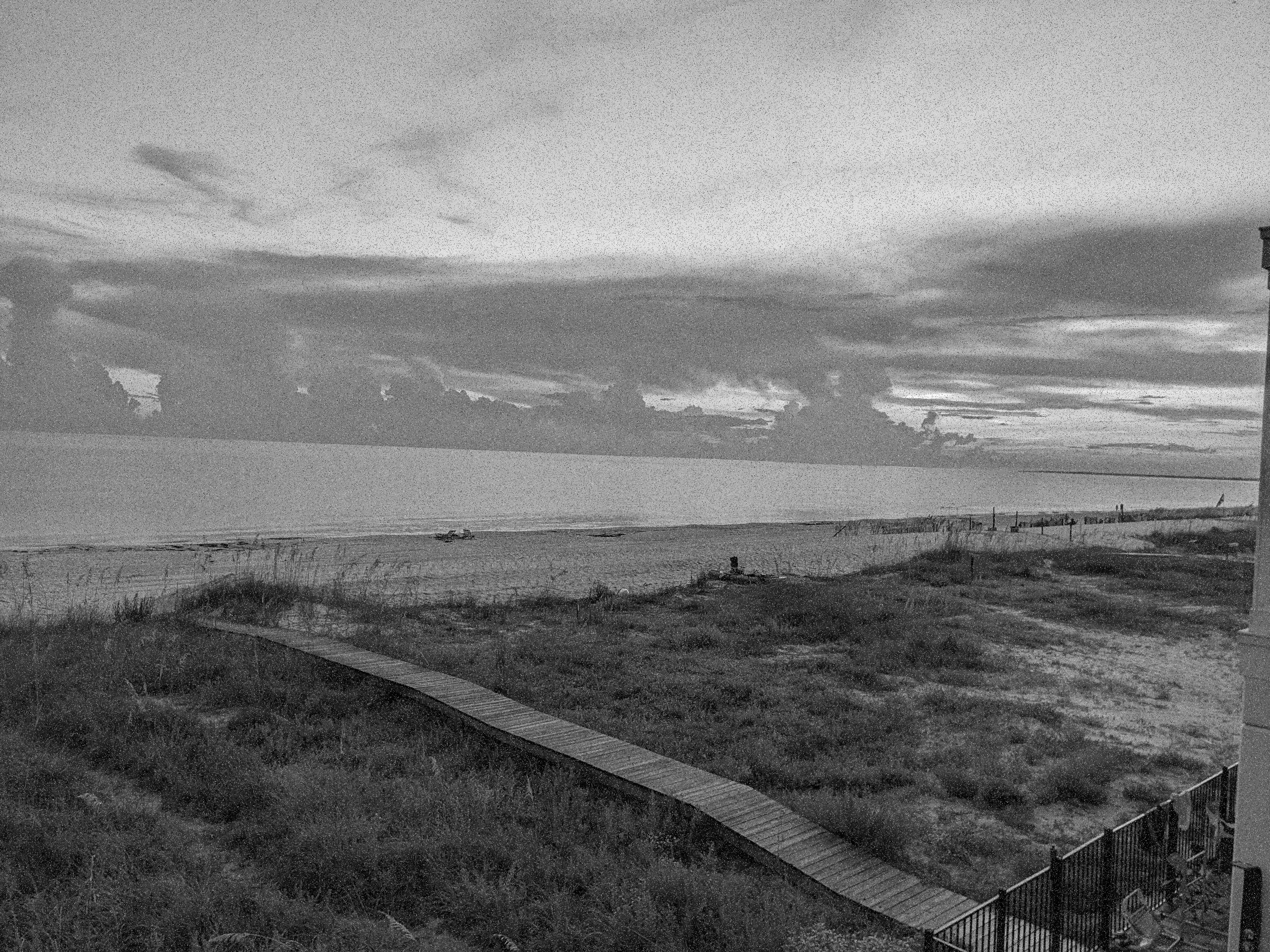
Salt & Pepper Noise
Salt and pepper noise is a specific type of noise found in grayscale images. It commonly occurs from data transmisson errors, and analog to digital conversion errors. Emulating this noise is a pretty easy:
- Grayscale the image if not already
- Decide how much of the image you want to be noise
- Generate a random pixel index
- Set the random pixel black for pepper noise, or white for salt noise
- Repeat until you've generated the wanted amount of noise
  // assumes image is grayscale

  FUNCTION salt_noise(noise_density)
    num_salt := noise_density * img_width * img_height

    FOR i TO num_salt
      // assumes range is inclusive
      rand_row := uniform_rand_int(0, img_height - 1)
      rand_col := uniform_rand_int(0, img_width - 1)

      img_data[img_width * rand_row + rand_col] := max_color
    END FOR

  END FUNCTION

  FUNCTION pepper_noise(noise_density)
    num_pepper := noise_density * img_width * img_height

    FOR i TO num_pepper
      // assumes range is inclusive
      rand_row := uniform_rand_int(0, img_height - 1)
      rand_col := uniform_rand_int(0, img_width - 1)

      img_data[img_width * rand_row + rand_col] := 0
    END FOR

  END FUNCTION
Warps
Flips
Flips are conceptually quite simple, but have some annoying index computations.
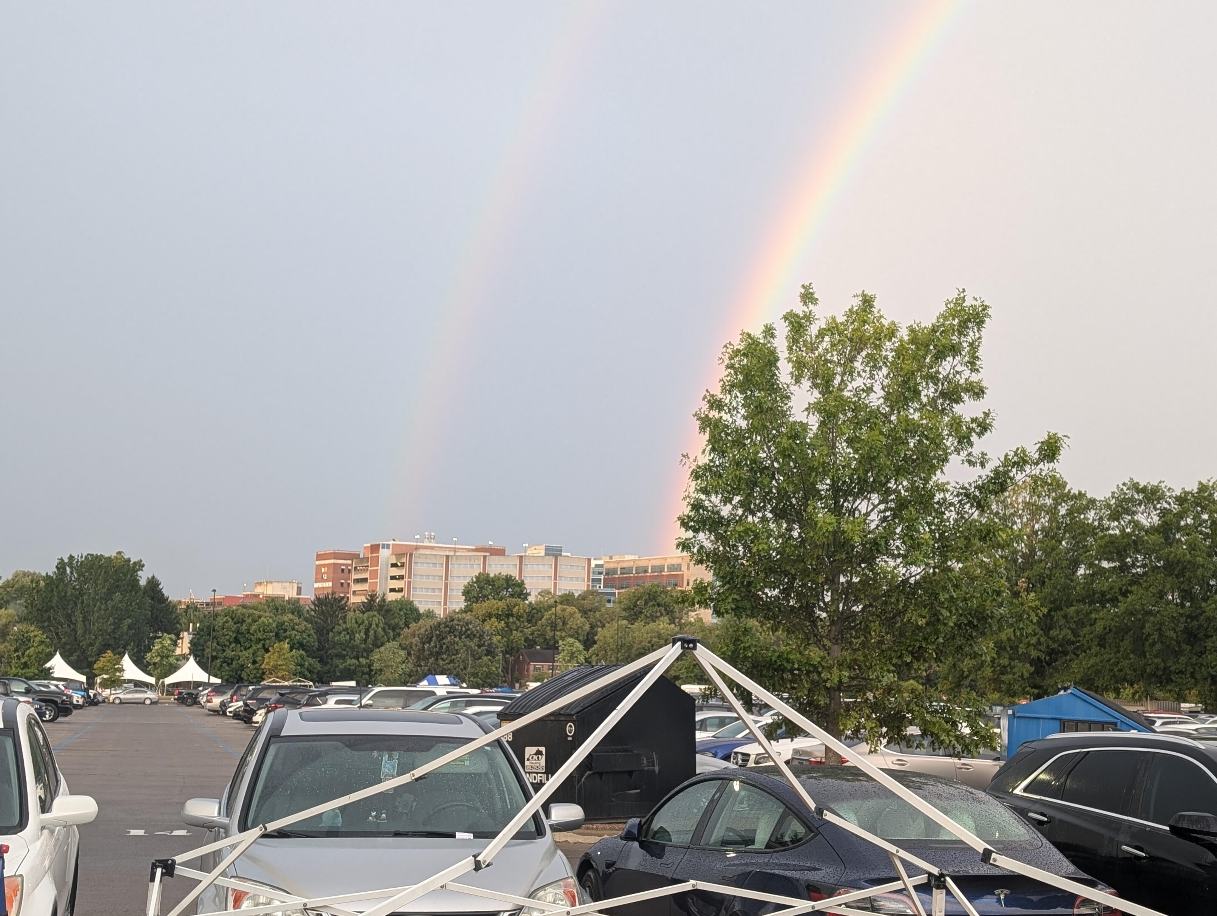
The first thing you need to do for both horizontal and vertical flips, is get the bounds you're iterating over correct. Given that these are symmetrical operations, you only need to iterate over half the image, calculating and swapping the current index with it's inverse position in the wanted dimension.
Calculating the left index in the horizontal case, and the top index in the vertical case is the same. You just use the standard calculation of \((width_{image} \cdot row + col) \cdot |channels|\).
The remaining two index calculations are bit tricky to come up with, so I recommend just performing the calculations on a matrix by-hand to understand all the details.
  FUNCTION horizontal_flip()
    FOR row TO img_height
      FOR col TO (img_width / 2)
        left_index := (width * row + col) * num_channels
        right_index := (( (width * row) + (width - 1) ) - col) * num_channels

        pixel_swap(left_index, right_index)
      END FOR
    END FOR

  END FUNCTION

  FUNCTION vertical_flip()
    FOR row TO (img_height / 2)
      FOR col TO img_width
        top_index := (width * row + col) * num_channels
        bottom_index := ( (height - row - 1) * width + col) * num_channels

        pixel_swap(top_index, bottom_index)
      END FOR
    END FOR

  END FUNCTION
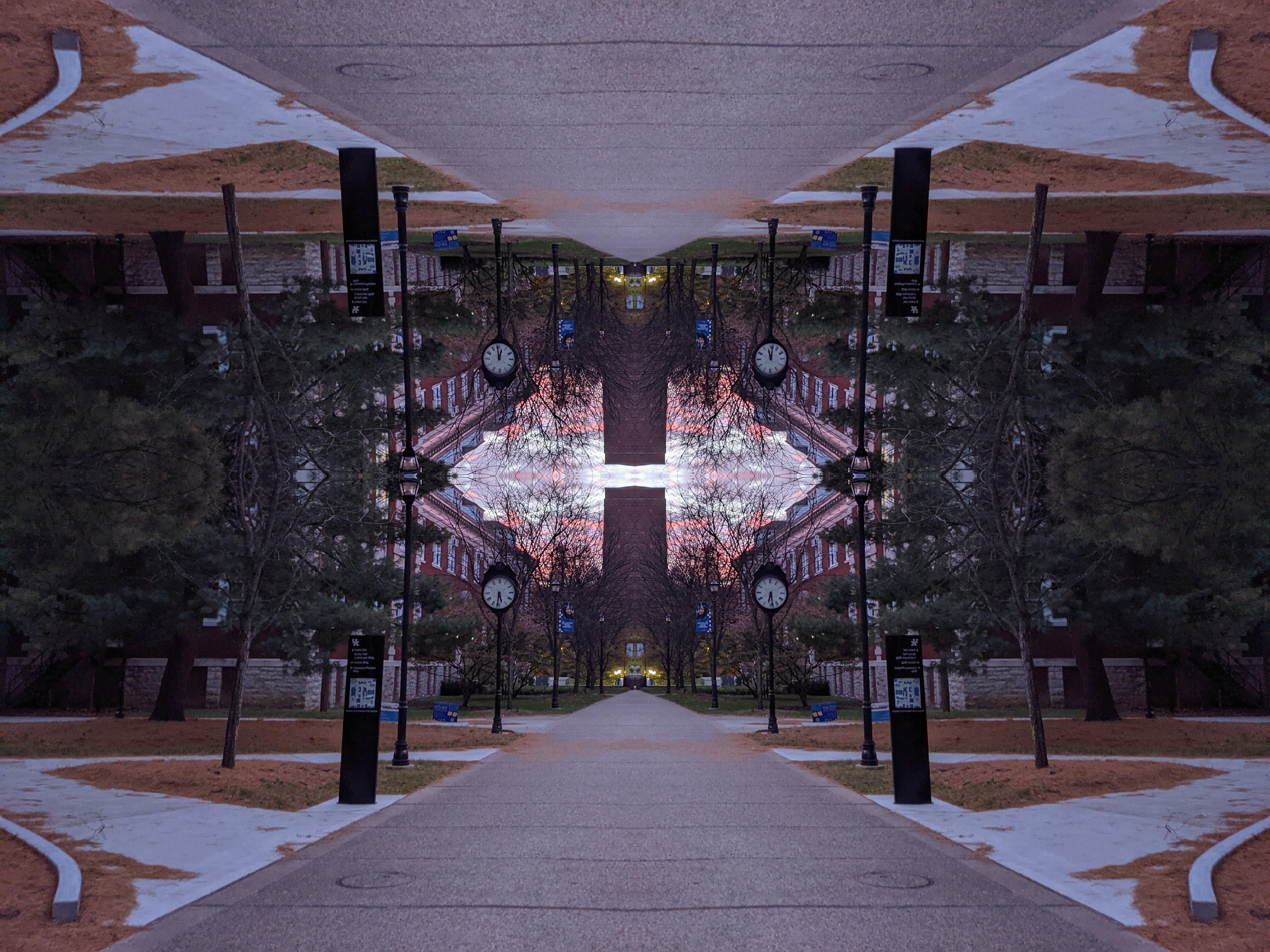
Reflections
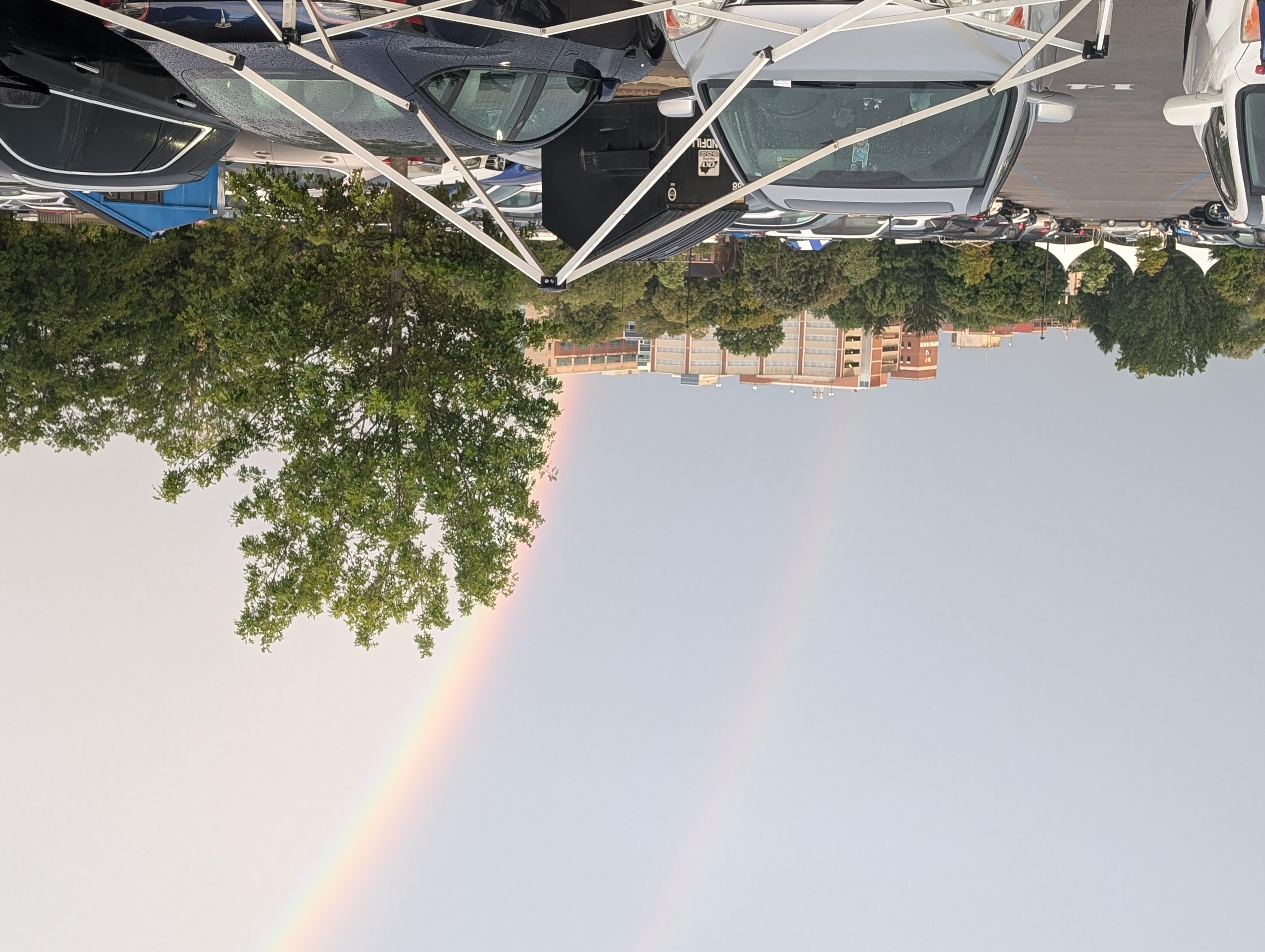
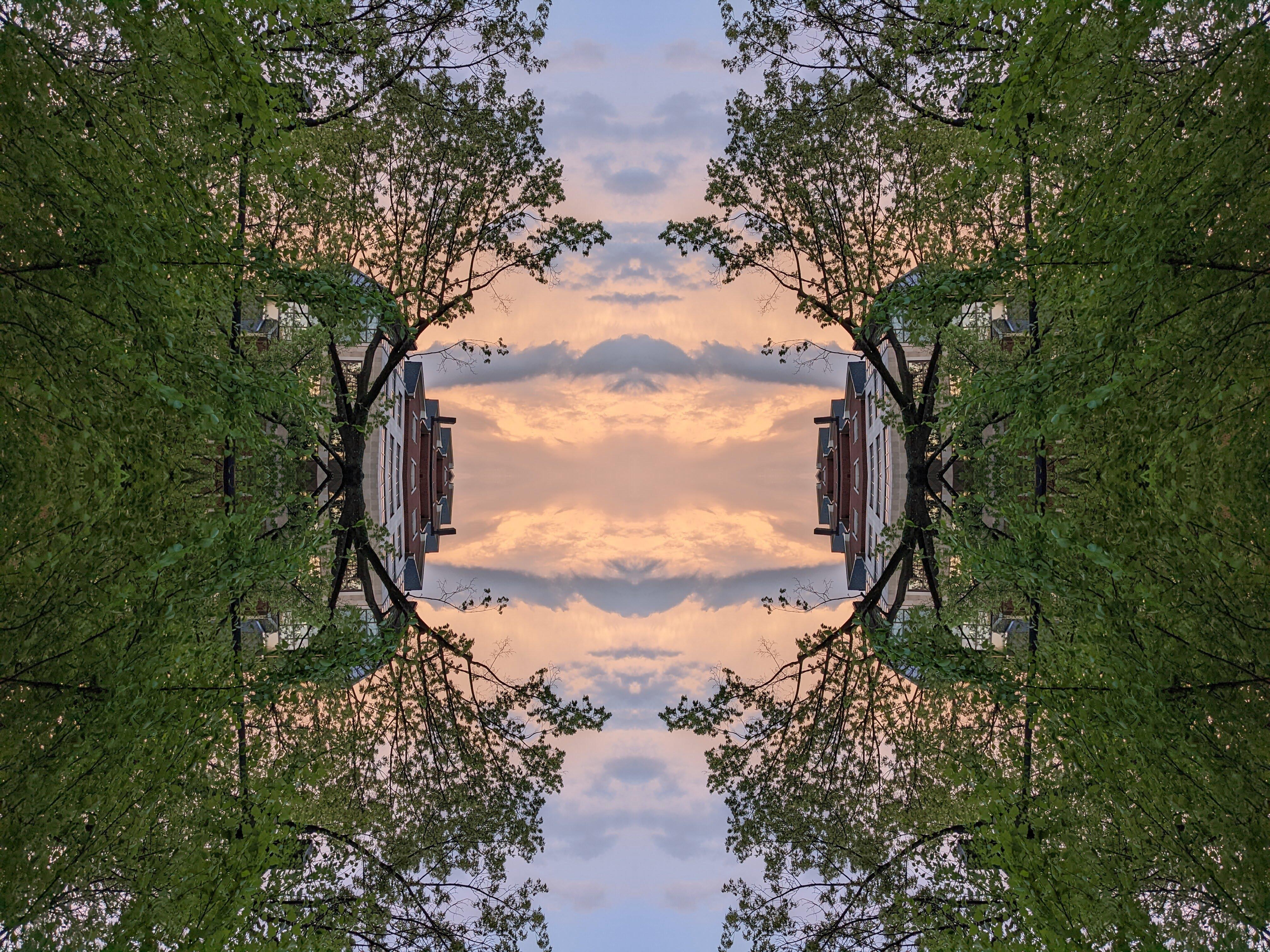
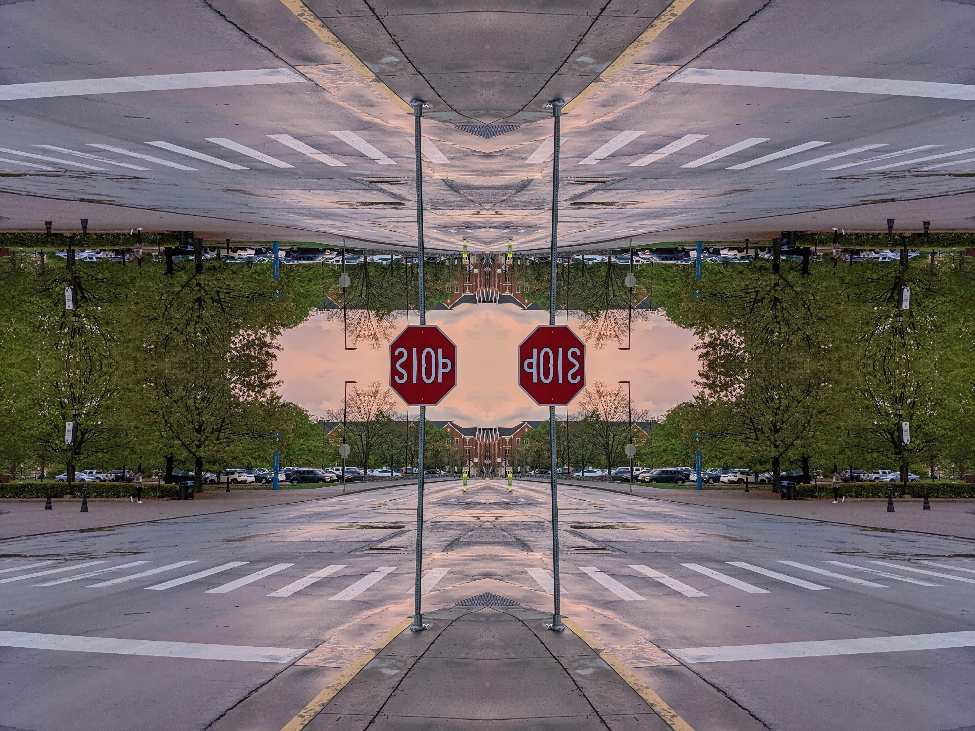
Of the image transformations I've implemented, reflections generate some of the most visually stunning images. And the nice thing is, if you've implemented the image flip algorithm's, you're basically already done. The only difference between flips and reflections is that you don't swap the computed indices, instead you simply override one with the other.
  FUNCTION horizontal_reflection(direction)
    FOR row TO img_height
      FOR col TO (img_width / 2)

        IF direction = 'L'
          FOR i to num_channels
            left_index := (width * row + col) * num_channels + i
            right_index := (( (width * row) + (width - 1) ) - col) * num_channels + i

            img_data[right_index] := img_data[left_index]
          END FOR
        END IF

        IF direction = 'R'
          FOR i to num_channels
            left_index := (width * row + col) * num_channels + i
            right_index := (( (width * row) + (width - 1) ) - col) * num_channels + i

            img_data[left_index] := img_data[right_index]
          END FOR
        END IF

      END FOR
    END FOR

  END FUNCTION

  FUNCTION verical_reflection(direction)
    FOR row TO (img_height / 2)
      FOR col TO img_width

        IF direction = 'T'
          FOR i to num_channels
            top_index := (width * row + col) * num_channels + i
            bottom_index := ( (height - row - 1) * width + col) * num_channels + i

            img_data[bottom_index] := img_data[top_index]
          END FOR
        END IF

        IF direction = 'B'
          FOR i to num_channels
            top_index := (width * row + col) * num_channels + i
            bottom_index := ( (height - row - 1) * width + col) * num_channels + i

            img_data[top_index] := img_data[bottom_index]
          END FOR
        END IF

      END FOR
    END FOR

  END FUNCTION
Rectangular Crop
Once again an image transformation whose main complexity stems from its index calculations.
There are more than one way to crop an image, this simple method only takes in the new origin point, and the new image dimensions. All you need to do is iterate over the new dimensions, and grab the pixels positions from the old image, using the new origin.
Once again to understand the calculation details, I'd recommend simply carrying out this operation on a matrix by hand.
  // assumes new origin is upper left corner of cropped image
  FUNCTION rect_crop(new_origin, new_width, new_height)
    new_img_data := ARRAY OF (new_width * new_height * num_channels)

    FOR row TO new_height
      FOR col to new_width
        old_index := ((new_origin[0] + row) * width + (new_origin[1] + col)) * num_channels
        new_index := (new_width * row + col) * num_channels

        new_img_data[new_index] = img_data[old_index]
        IF num_chanels = 3
          new_img_data[new_index + 1] := img_data[old_index + 1]
          new_img_data[new_index + 2] := img_data[old_index + 2]
        END IF
      END FOR
    END FOR

  END FUNCTION
Scaling
Image scaling is a classic example of being quite simple once you know the correct answer, but can be dubious otherwise.
The first step is obvious, let's compute the dimensions of the new image using our scale factors. Now let's take the logical next step, for each pixel in the unscaled image, map it to the new image by multipling it's indices by their respective scale factors.
Bam, done, all the pixels have been mapped from the old image to the new. And while this is true, if you think about what you've done, you'll realize most of the new image is empty.
The problem here being your intution, as if it's lead you down this path, you've been lead astray. While maybe unintutive, what you need to do is work backwards from the empty scaled image. More specifically, iterate over the empty scaled image, and multiply each pixel's coordinates by the inverse of their respective scale factors. Now use this to index into the original image, and set your new pixel to that pixel.
The only issue with this method is that you will get decimal index value's, you can deal with this by simply rounding, or taking the floor of the index. It should also be noted that this technique is called nearest neighbor interpolation, and there are other more advanced methods which result in smoother scaling. However as of yet I haven't had the time to implement them, so I won't be going over them until then.
  FUNCTION scale(width_scale_factor, height_scale_factor)
    new_width := img_width * width_scale_factor
    new_height := img_height * height_scale_factor

    inv_width_scale_factor := 1 / width_scale_factor
    inv_height_scale_factor := 1 / width_height_factor

    new_img_data := ARRAY OF (new_width * new_height * num_channels)

    FOR row TO new_height
      FOR col TO new_width
        new_index := (new_width * row + col) * num_channels

        // nearest neighbor interpolation
        old_row_index := round(row * inv_width_scale_factor)
        old_col_index := round(col * inv_height_scale_factor)
        old_index := (img_width * old_row_index + old_col_index) * num_channels

        new_img_data[new_index] := img_data[old_index]
        IF num_channels = 3
          new_img_data[new_index + 1] := img_data[old_index + 1]
          new_img_data[new_index + 2] := img_data[old_index + 2]
        END IF
      END FOR
    END FOR

    img_data := new_img_data
    img_width := new_width
    img_height := new_height

  END FUNCTION
Additional Image Processing Resources
If you want a more formal understanding of image processing the Gonzalez & Woods textbook is to my understanding the standard textbook for image processing; personally I’ve been going through it and it’s been very good. There’s also some great lectures on YouTube by Rich Radke, which go over a good portion of the book. With that being said the content is not the most easily digestible, especially if you haven’t taken college level math courses.
The YouTube channel ComputerPhile has an image processing playlist that is quite good; their channel is also a great resource for a variety of CS related topics. If you’re more interested in artistic image processing, The Coding Train is a treasure trove of artistic image manipulations and animations.
Finally the last resource I have to recommend is ChatGPT. If it generates code for you there’s a good chance it won’t work, and it may get small details wrong, but I’ve found it the best place to start when researching how to create a certain effect. Usually I use it as jumping off point to dig deeper into a topic, as it gives you enough background information to more easily search google, and understand more technical articles.
