Background
Last summer I worked at the University of Kentucky's KAOS research lab, which specializes in efficient/parallel computing and computational photography. Under the direction of Prof. Dietz, my project was to optimize KEMY (Kentucky Error Modeler) a specialized image denoiser. My work resulted in KEEMY (Kentucky Efficient Error Modeler), which significantly reduces runtime while improving denoising quality.
KEMY is a Non-Local Means (NLM) style denoiser that leverages a statistical error model to determine patch similarity. While I go into all the details after the results section, the primary bottleneck in KEMY is the high computational cost of this custom similarity metric. To overcome this, KEEMY is a complete rewrite of the denoising pipeline, utilizing the PatchMatch algorithm and an image pyramid to optimize the search process, thereby reducing similarity computations.
The code for this project is publicly available on my github.
Results
PC Hardware
For additional context the CPU is a mid-tier chip from ~8½ years ago.
Denoiser Speed Comparison
| Threading | Wall Time | Memory |
|---|---|---|
| Multi (6) | 00m 32.58s | 10.95GB |
| Single | 01m 58.67s | 10.95GB |
| Threading | Wall Time | Memory |
|---|---|---|
| Multi (6) | 02m 42.82s | 0.30GB |
| Single | 15m 24.17s | 0.30GB |
| Threading | Wall Time | Memory |
|---|---|---|
| Multi (6) | 11m 12.63s | 18.87GB |
| Single | 51m 42.19s | 18.86GB |
| Threading | Wall Time | Memory |
|---|---|---|
| Multi (6) | 00m 11.10s | 0.48GB |
| Single | 00m 45.92s | 0.43GB |
| Program | Threading | Wall Time | Peak Memory |
|---|---|---|---|
| KEEMY | Multi (6) | 00m 32.58s | 10.95GB |
| Single | 01m 58.67s | 10.95GB | |
| KEMY | Multi (6) | 02m 42.82s | 0.30GB |
| Single | 15m 24.17s | 0.30GB | |
| BM3D | Multi (6) | 11m 12.63s | 18.87GB |
| Single | 51m 42.19s | 18.86GB | |
| NLM | Multi (6) | 00m 11.10s | 0.48GB |
| Single | 00m 45.92s | 0.43GB |
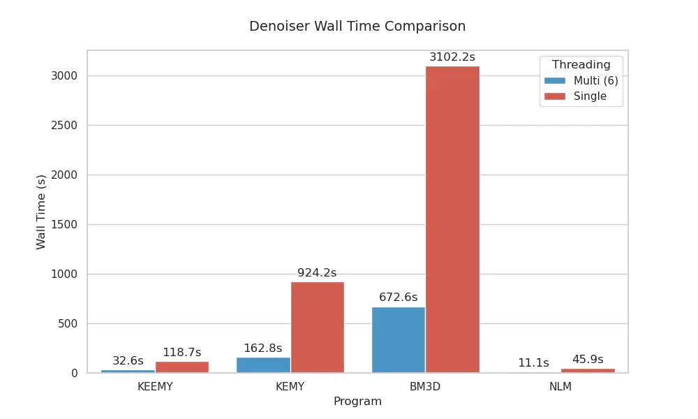
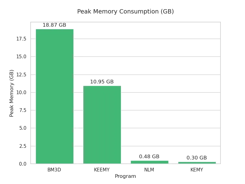
The benchmark DPReview test image is a naturally noisy 51884 x 3888 image. Also, the C++ NLM and Python BM3D implementations were sourced from OpenCV and the official Python package, respectively; you can download the denoiser scripts here. It should also be noted that KEEMY and KEMY use their default parameters.
As you can see from the benchmark KEEMY is significantly faster than KEMY: in multithreaded scenarios KEEMY is 5.00x (399.75%) faster and in single-threaded 7.79x (678.77%) faster. In fact, single-threaded KEEMY is 1.37x (37.20%) faster than multithreaded KEMY. Of course the primary drawback is its memory usage, however the memory footprint is still significantly smaller than BM3D's.
Image Quality Comparisons
The How it Works section explains KEEMY parameters in detail, but here is a quick reference:
| Parameter | Default | Recommended | Effect |
|---|---|---|---|
| K_MAX | 40 | 30-80 | Number of similar patches stored per-pixel. Directly scales memory usage and denoising quality, however too high of a value can over smooth images; comparison here |
| denoisePasses | 2 | 1-5 | Number of times the denoise function is run. Higher values increase smoothness, but excessive passes may cause posterization; comparison here |
| simContributionThresh | 0.00 | 0.00-0.06 | Threshold for pruning tail of patch matches. Higher values better preserve fine detail, but can increase noise; comparison here |
DPReview
The figure below compares the DPReview image outputs from the speed benchmark.
For accurate comparison images are lossless; loading may be slow.

As you can see, there are some trade-offs with KEEMYs quality as opposed to KEMYs; KEEMY does a better job at getting rid of noise, but in high-detail areas it can lose some detail. It's also pretty clear that BM3D has the best fine detail preservation, although it's not better across the board. NLM on the other hand just generally does a pretty terrible job; NLM is mainly included given its conceptual similarity to KEEMY/KEMY.
It's also important to keep in mind that while BM3D is generally considered the gold standard for non-ML(machine learning) denoising, it is designed to work best with additive white Gaussian noise (AWGN); there are BM3D variants which work with other kinds of noise, but you have to know the noise type before-hand. This also means BM3D doesn't work very well when image noise comes from multiple different sources.
NIND
The DPReview image is a great test image, but it's taken in a controlled environment unlike real-world images. Furthermore, you need more than one example image to evaluate a denoiser's general ability. As such, I've also included a comparison of 15 images from the Natural Image Noise Dataset (NIND).
For the below NIND comparison I've frozen each denoiser's parameters so they're the same across all images. This means the comparison does not represent the best any of the denoiser's can do, but it is representative of real-world batch denoising use; tuning each denoiser for each image is impractical and subjective. In addition, I've replaced NLM with a modern ML denoiser SCUNet, as NLM has no chance of beating any of the other denoisers.
KEMY uses the default parameters as there are none to tune. KEEMY uses the following: K_MAX=60, denoisePasses=4, and simContributionThresh=0.02. BM3D uses Sigma=0.15, as MAD estimation proved to be useless. SCUNet uses the PSNR checkpoint as the GAN checkpoint purposefully hallucinates texture, with: tileSize=512, tilePadding=32.
For accurate comparison images are lossless; loading may be slow.
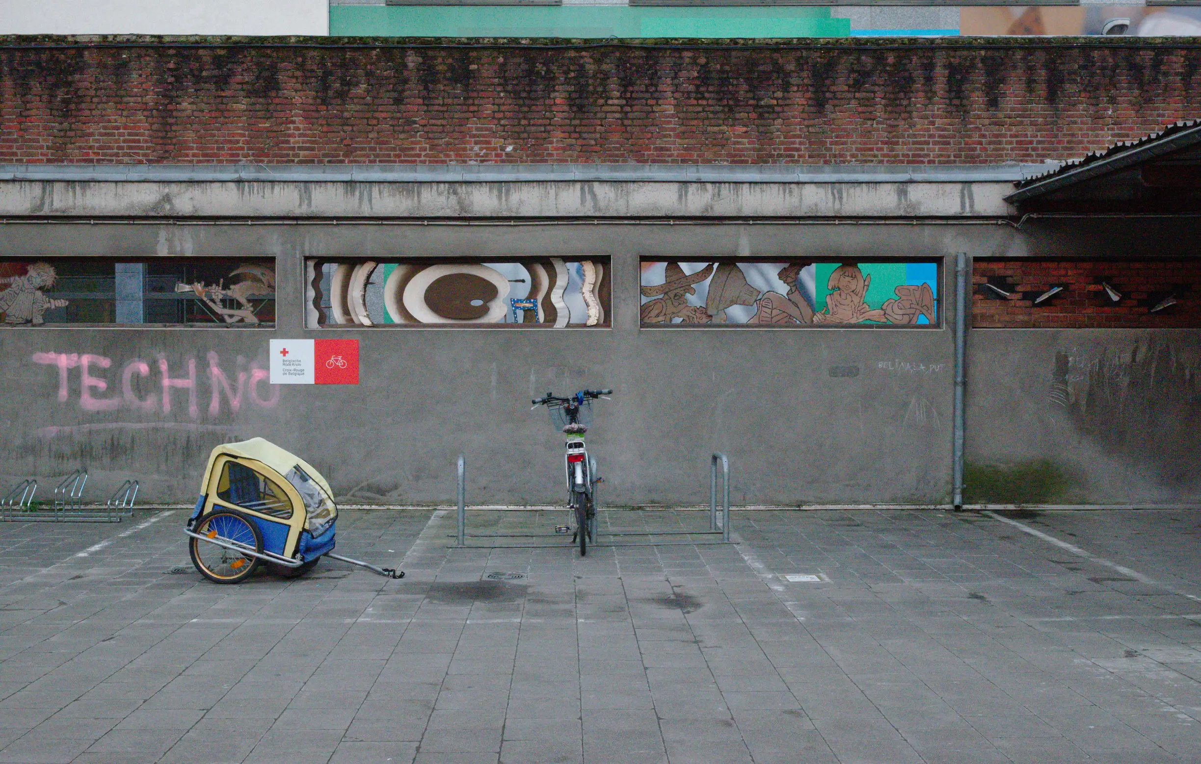

The NIND comparison really highlights KEEMYs improvements over KEMY, as well as BM3Ds inability to denoise in complex real-world scenarios. Furthermore, while SCUNet is definitely the best performer (this is expected) KEEMY still looks quite good in comparison, even outperforming it in certain instances. This is especially impressive when you take into account KEEMY is running quite quick on an old CPU, whereas SCUNet requires a good modern GPU. With that being said, under extreme noise SCUNets performance is far and away the best.
ML Denoising Issues
As seen in the NIND comparison SCUNet performs incredibly well, but if you look closely you'll find some hallucination / aberrant blurring issues. While these issues are in SCUNet, they're more issues inherent with the ML approach.
It's important to remember when a pixel is noisy there's no way of knowing exactly what its value should be, so hallucination is inherent to the denoising process. However, if the image you're denoising does not have representative content in the training dataset, the hallucinated output won't either. On the other-hand, in instances where there's lots of noise and little signal, training off of many images allow ML denoisers to hallucinate reasonable textures which wouldn't otherwise be possible.
While you can find hallucination issues in the SCUNet NIND images, I found a very noisy example image that really illustrates these issues. The comparison below is of two ML models: SCUNet and Restormer, as well as the traditional KEEMY and BM3D methods; the image was taken from this article by Spencer Cox.
For accurate comparison images are lossless; loading may be slow.

If you look at the bushes to the left of the main two rocks, you'll see that Restormer and SCUNet replace it with incorrect textures; Restormer seems to have replaced the bushes with a rock texture, and SCUNet heavily distorts the textures. There is more SCUNet distortion and incorrect Restormer texture replacement around the short dead tree on the left. Furthermore, Restormer replaces the bushes on the extreme right of the image with a rock texture.
While I completely understand preferring either of the ML methods over either of the traditional, the hallucination issues can be seriously problematic depending on your use case, specifically applications like medical imaging, crime photos, etc.
Now of course I've painted with broad strokes here, as there are many different kinds of ML denoisers; some of the most cutting-edge denoisers use self-supervised or 'zero-shot' techniques which can train solely on the image you're denoising, similarly to KEEMY/KEMY. However, in-practice single image training currently has speed and quality issues, so most self-supervised denoisers still generalize from a dataset. With that being said, I expect these single image training issues to be ironed out in the future.
How it Works
This explanation assumes little to no prior knowledge of image processing; I want to provide enough information and resources that any developer can understand this project. As such, if you already have a background in image processing, you can skip straight to the KEMY explanation.
General Denoising Background
Image Noise
A pixel is considered noise if it does not accurately represent the content of a scene. While noise comes about from a variety of different sources, it's best understood as visual errors or anomalies captured during the imaging process.
There is however one very important characteristic of noise, its stochastic nature; if you're unfamiliar with the term 'stochastic', it just means a random process. This is important as it means two noisy images taken of the same content, with the same camera location, may have different noisy pixels.
Image Stacking (Denoising Gold Standard)
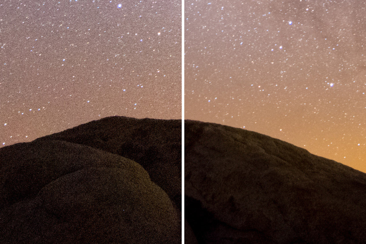
Image stacking is different from the Non-Local Means style denoising of KEEMY, however it provides a great framework to understand it from.
As mentioned above, if you take two photos of the exact same scene, the noise will appear differently in each image. This means if you look at any given pixel across both images, there’s a chance that in one image it will be noise, whereas in the other it will represent the true scene content.
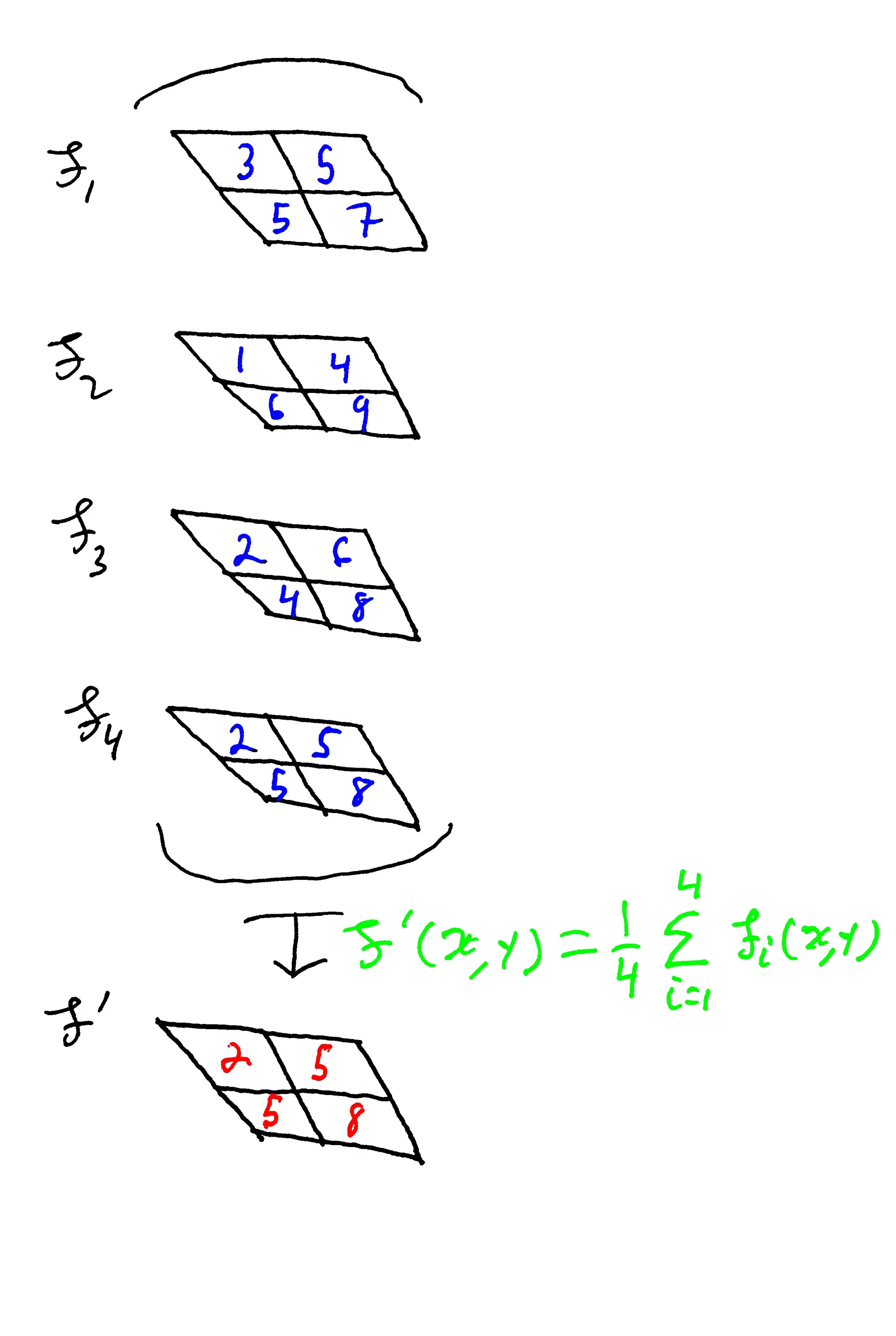
This idea forms the basis for image stacking; instead of taking a single photo, you record multiple frames of the same scene and then align, or “stack”, them. Denoising is then performed by “blending” the frames together, as the true image content is consistent while noise varies randomly between frames. To be more specific, the blending process typically takes the mean or median of each pixel at the same position across all frames; if you’ve ever used the night-sight feature on your phone, this is one of the things it’s doing, and why it asks you to keep your phone very still.
An aside but related, adobe has an interesting experimental photo app (project Indigo) which among many things, always utilizes image stacking.
Non-Local Means (NLM)
So as I’ve covered, image stacking is the gold standard for image denoising. However, most of the time you only have a single image to work with. If this is the case, let’s think about how we could approximate the image stacking technique.
The key idea behind Non-Local Means (NLM) is to look for similar scene content within the same image; in image stacking the same content is taken directly from other scene samples, but we can approximate this by looking for similar content in our one scene sample. More formally, this approaches exploits natural image self-similarity.
Unlike image stacking, which compares a single pixel across multiple frames, NLM requires a broader "context" to identify whether the pixels represent similar scene content; this isn't necessary in image stacking because frame alignment ensures corresponding pixels represent the same content.
To denoise a specific target pixel, the algorithm first extracts a small reference patch (context) centered around it (typically 3×3 to 7×7 pixels). Then for all other pixels in the image, a centered patch is extracted and its similarity to the reference patch is determined. The new value for the target pixel is calculated by averaging together the center of all pixel patches, but weighted according to patch similarity. The effect of this, is moving the average towards pixel values in the best matches, without completely discounting patches that don't perfectly match up.
This process is repeated for every pixel, with updates written to a separate output image as to not intermix source and denoised data. For color images you have three channels, so this process is performed independently in each channel. The overarching idea is to effectively "stack" an image against itself, leveraging natural content repetition to average out noise.
From here there are two algorithmic points to consider:
- How do we determine patch similarity?
- How do we deal with the fact that comparing every pixel patch to every other is generally intractable?
Frobenius Norm as Similarity
*Note you need to have a basic understanding of vectors and matrices to understand the similarity metric.
NLM quantifies similarity between two patches as the squared distance between them, in the pixel value domain. This is a bit strange, as what does it mean to take the distance between patches?
The patches of pixels are really matrices, so the question is really how do you get the magnitude of a matrix; distance is the the magnitude of difference between matrices/vectors.
There are many methods for calculating matrix magnitude, but the frobenius norm is the standard one given it's an extension of the standard vector norm (L2). It's very easy to calculate, you just flatten the matrix into a vector and then use the standard method of the Pythagorean theorem.
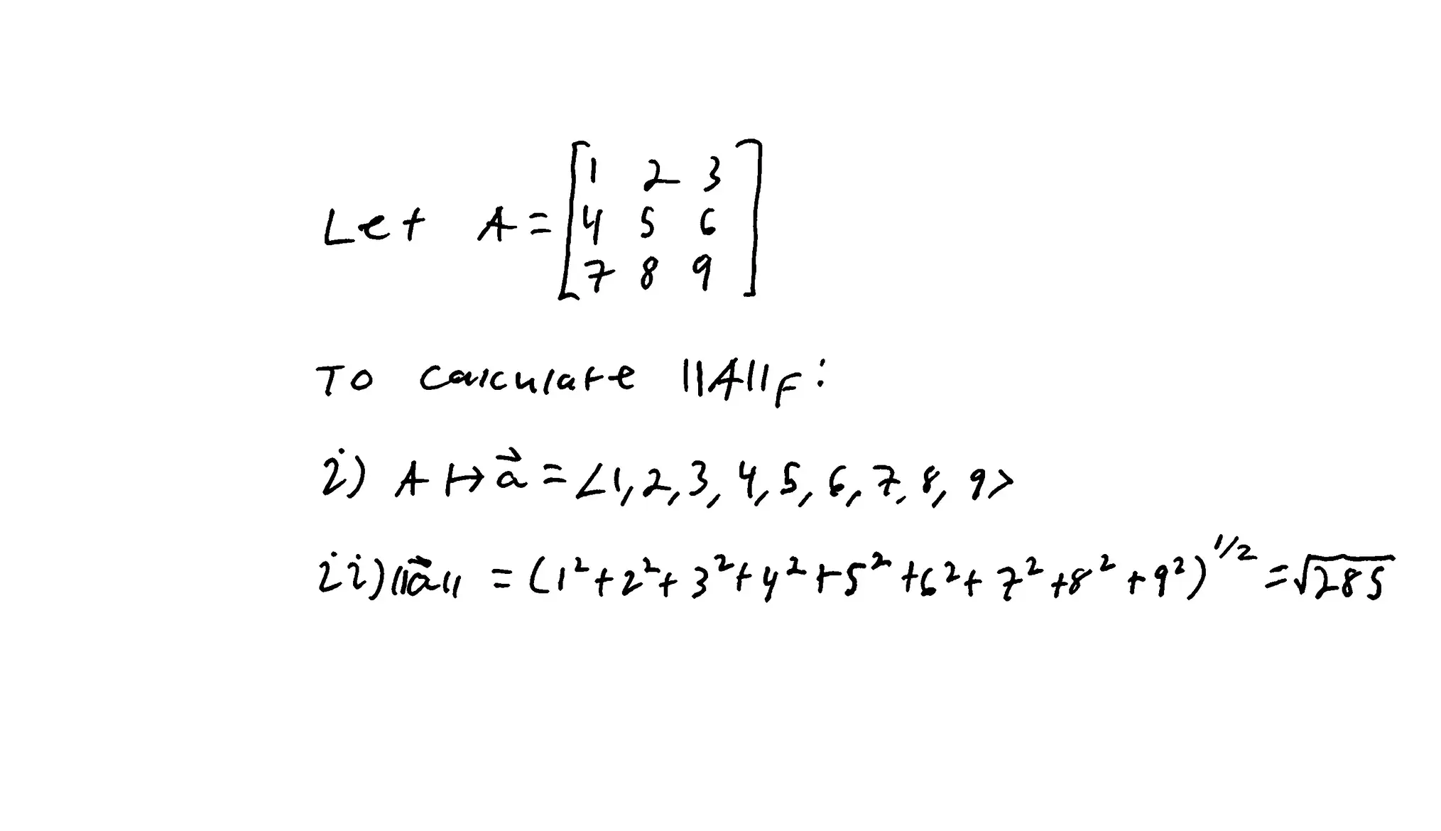
Geometrically what you're doing is treating each element as its own dimension. This means for an n by m matrix, you're operating in an \(n \cdot m\) space. Also, remember the similarity isn't distance but squared distance; by squaring distance we penalizes matches more harshly the further away they are.
Search Window
If for each target patch we were to extract and compare every other patch, the complexity is: \(O(N^2 \cdot K) \text{ where } K \text{ is pixels in a patch}\). As an example, for a standard 1080p image using only 3x3 patches: \(O(38,698,352,640,000)\) per-channel, so really \(O(116,095,057,920,000)\). And this is only for 1080p images, even crappy modern phones shoot 4k.
The solution to this is pretty straightforward, instead of comparing the reference patch to every other patch, you limit the search to a window (typically 21 x 21) centered around the target. This turns the complexity calculation to: \(O(N \cdot S \cdot K ) \text{ where S is search pixels}\), so including the per-channel calculations the above example turns into \(O(24,690,355,200)\). This all works by leveraging the generally good assumption that pixels close to each other represent similar content, however it does significantly limit the patch candidate pool.
If you find the name Non-Local Means confusing in light of this, you aren't alone, the researchers agree; here is a direct quote from page 2 of the original 2011 paper: "Since the search for similar pixels will be made in a larger neighborhood, but still locally, the name “non-local” is somewhat misleading. In fact Fourier methods for example are by far more nonlocal than NL-means. Nevertheless, the term is by now sanctified by usage and for that reason we shall keep it."
NLM Algorithm Visualization
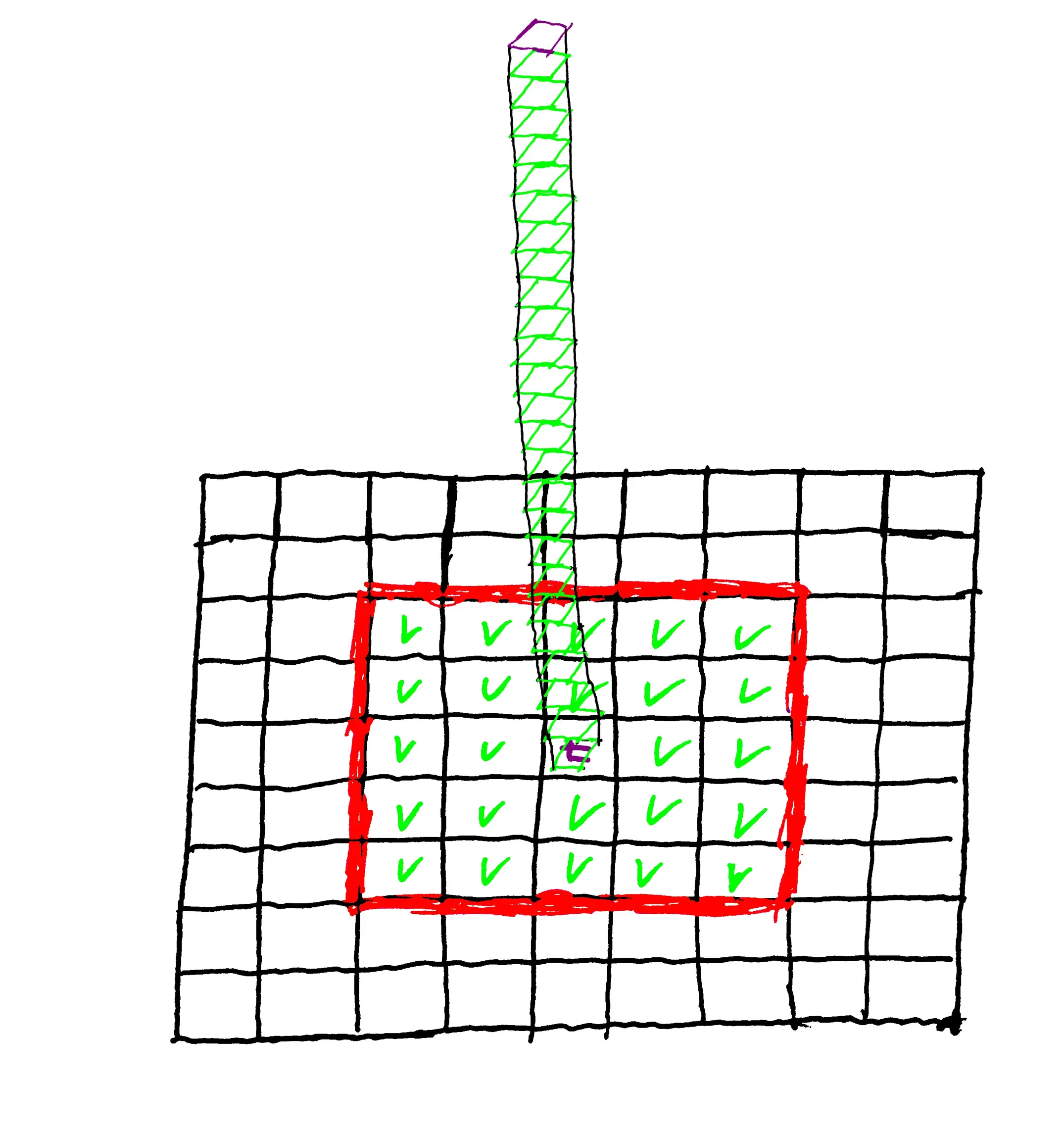
If you're confused about the diagram, it shows the process of denoising a single target pixel. First, you extract the patch (patch boundaries aren't shown for clarity) around the 't' pixel, then you extract a patch centered around all the other pixels in the window (v's). You then calculate the similarity from the t patch to each of the v patches. Finally, you conceptually stack the patches above the t pixel and blend the center's together to determine t's denoised value.
Full NLM Denoise Computation
I haven't described all the NLM denoising calculations as they aren't important for understanding KEEMY or KEMY, but I'd be remiss if I didn't include them.
- Image Domain
- \(\text{Let } \Omega \subset {ℕ}^2 \text{ be the Image Domain}\)
- Intensity Map
- \(\text{Let } I: \Omega \to {ℕ} \text{ be the Pixel Intensity Map}\)
- Search Window
- \(\text{Let } S \subseteq \Omega \text{ be the Search Window} \)
- Patch Matrix
- \(\text{Let } P \text{ be a Patch Matrix} \)
- Target Pixel
- \(\text{Let } t \in \Omega \text{ be the Target Pixel Index}\)
- Smoothing Parameter
- \(\text{Let } h \in {ℝ} \text{ be the Smoothing Parameter}\)
-
\(w(t,i) = \exp\left( -\frac{\| P_t - P_i \|^2_F}{h^2} \right)\)
-
\(Z(t) = \sum\limits_{i \in S} w(t,i)\)
-
\(I(t) \leftarrow \left\lfloor \frac{1}{Z(t)} \sum\limits_{i \in S} w(t,i) \cdot I(i) \right\rfloor\)
It should be noted that the original paper also used a Gaussian kernel to weight the distance computations, but it's seldom done in practice.
KEMY Explanation
Before diving into how KEMY works, it should be noted that KEMY is actually a port of KREMY, which is conceptually the same except it works on raw images; the performance issues with KEMY stem from having to process three separate channels, essentially tripling the work. I bring this up because if you understand KREMY you understand KEMY, and Prof. Dietz published a paper on KREMY you can find on this page, as well as a webpage on KEMY. In addition, he recently published a paper further exploring statistical error models, which you can find here.
I highly recommend looking over the above resources, as I won't be deep-diving into the statistical model; if you want a really deep understanding of the statistical model and the surrounding theory, read the papers.
Statistical Error Model
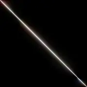
KEMY/KEEMY use a statistical error model built from pixel-pair frequencies to derive their patch similarity metric. The benefit of this, is that the metric is incredibly discriminative and able to semantically understand image content as well as noise in a way the traditional squared distance method can't.
In the above visualization/graph, the x-axis represents values observed by the camera, and the y-axis represents the accurate/true values. This means the white line is where the observed values match the true values, with the off-diagonal pixels representing instances where the observed values differ from the truth; the color is because each color channel has its own error model, so color shows in which channels errors are occurring.
Building the Error Model
The model works off the assumption that at least one of a pixel's eight neighbors represents the true scene content, differing only by noise. As such, the basis of the model is a 2D histogram where each possible pixel value has its own bin in each dimension (x for observed, y for truth). To populate the histogram, the difference in value is computed between each pixel and its eight neighbors. If the neighbor closest in value is below a threshold, the algorithm performs a "square bump".
In this square bump, the algorithm increments every bin in the 2D histogram that falls within the range between the observed value and the truth value. For example, if the observed pixel is 100 and the neighbor is 102, all coordinates in the $3 \times 3$ grid from 100 to 102 are incremented. The reason is that if these two readings likely represent the same scene content, then every integer value in the span between them is also a statistically credible candidate for the truth.
After the histogram is fully populated monotonicity is enforced; monotonic enforcement ensures the further away the observed value is from the truth, the smaller the probability, and the closer the observed value is to the truth, the larger the probability. Finally, the histogram is converted into a normalized probability density function (PDF) by scaling each row independently so the maximum probability is 255; scaling each row to \([0, 255]\) instead of \([0, 1]\) allows the model to function as a fast lookup table.
Deriving Similarity from the Model
There are two similarity functions derived from the error model: similarity and simPatch
- similarity is the similarity between two pixels directly from the error models; in each channel you lookup the similarity between the pixel values, then multiply the results together (the per-channel probabilities are independent).
-
simPatch is the similarity between two patches; the similarity function is only ever called inside simPatch as patch similarity is ultimately what we want. Computing patch similarity is a bit more involved as it's the multiplication of three terms: \(s^2\), \(best\), and \((best_1)^2\).
- \(s\) is the similarity between the patch centers.
- \(best\) is the most similar pair of adjacent pixel pairs between patches.
- \(best_1\) is the most similar pixel pair between patches.
similarity(pixel_t *a, pixel_t *b) {
  // how similar are these multi-color pixel values?
  return (PDF(0, a[0], b[0]) * PDF(1, a[1], b[1]) * PDF(2, a[2], b[2]));
}
simpatch(pixel_t *a, pixel_t *b) {
  // compute similarity of patches around a and b
  float sim[POFFS + 1];

  for (int i = 0; i < POFFS; ++i) {
    sim[i] = similarity(a + poff[i], b + poff[i]);
  }
  sim[POFFS] = sim[0];

  // find highest combined similarity of two adjacent neighbors
  float best1 = sim[0];
  float best = sim[0] * sim[1];
  for (int i = 0; i < POFFS; ++i) {
    float s = sim[i] * sim[i + 1];
    if (s > best)
      best = s;
    if (sim[i] > best1)
      best1 = sim[i];
  }

  // return best weighted by similarity of a and b
  // this determines number of PDF terms multiplied:
  // best1 and s are 1 similarity each, best is 2
  // and each similarity is 3
  float s = similarity(a, b);
  return (best1 * best1 * best * s * s);
}
Denoising Method
KEMY denoises similarly to NLM, it blends similar patches together in a search window (search window is a disc shape) around the current pixel. However, the patches are weighted by the similarity metric derived from the custom error model, as well as L2 distance; L2 distance weighting increases blending strength given the constrained search and further emphasizes spatial coherence.
Problems with KEMY
The problem with KEMY is not its denoising ability, although KEEMY does further improve it, it's the runtime on large images; its worth optimizing for larger images as even smartphones typically shoot 4k+. Furthermore, Prof. Dietz who wrote KEMY specializes in performant computing, so while there may be some performance left on the table, its non-obvious and most-likely insufficient; the real performance killer is not the implementation, but the complexity of simPatch.
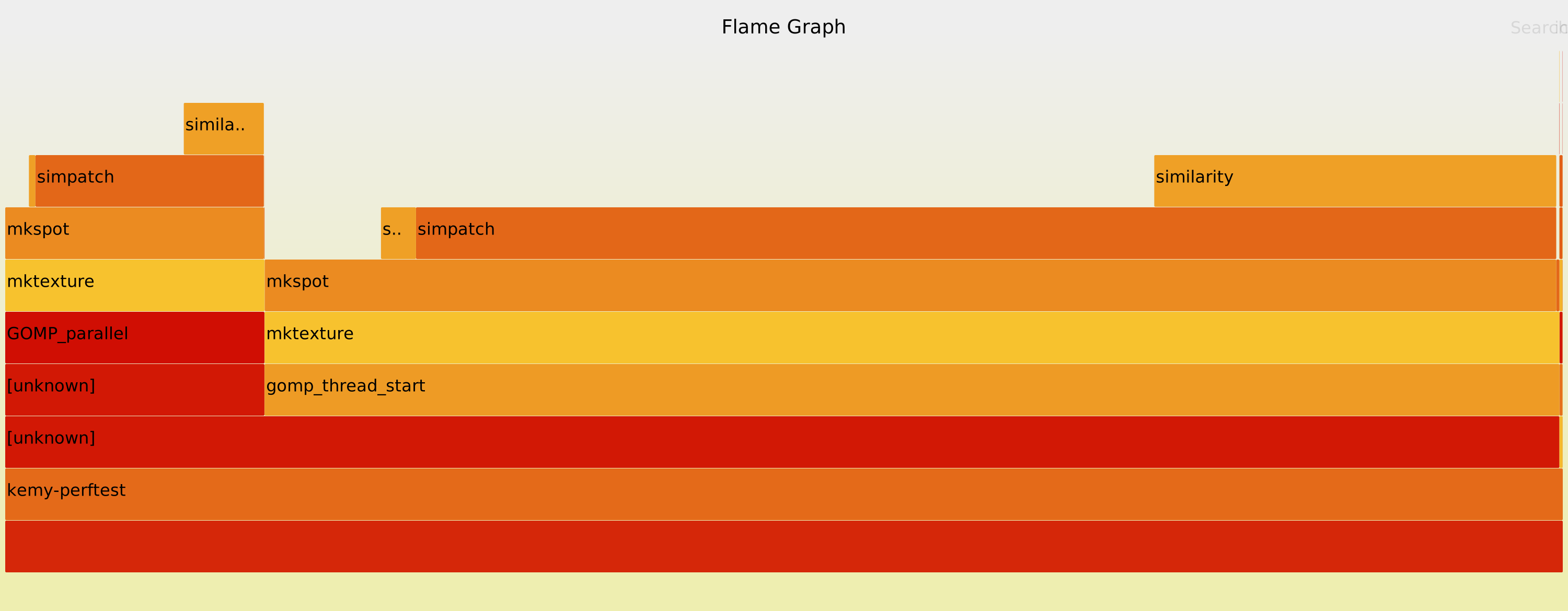
This is why KEEMY retains all the error model and similarity code but rewrites everything else, to fundamentally reduce the number of necessary simPatch calls.
KEEMY Explanation
Both KEMY and NLM follow the same general steps: for each pixel perform a local patch search and utilize the patches to denoise the current pixel. KEEMY on the other-hand works slightly differently:
- PatchMatch Algorithm: Find and store the \(k\) most similar patches for all pixels
- Weighted Average: Denoise each pixel using it's top-\(k\) patch stack
The main downside of this approach is memory usage; storing the location and similarity of \(k\) patches for every pixel is memory intensive, for large images and/or \(k\).
PatchMatch
The PatchMatch algorithm was created through collaboration between researchers at Princeton and Adobe, originally published in 2009. You can read the original paper here , as well as the follow-up paper in 2010 which further generalizes the algorithm. It's been used for a variey of applications, many of which are showcased in this Adobe demo video and this blog post.
There are a variety of different algorithms for finding approximate nearest neighbors (ANN), but I chose PatchMatch for a couple reasons:
- The algorithm has no constraints on the search metric e.g. triangle inequality
- The search efficiency significantly reduces the number of similarity calls
- The algorithm improves match quality through global search (actually non-local)
The PatchMatch algorithm has three main steps, with the second and third repeating \(n\) times.
- Offset Initialization
- Propagation (local search)
- Random Search (global search)
initialize_offsets(img)

global_radius_x := floor(img_width / 2)
global_radius_y := floor(img_height / 2)

FOR n FROM 0 TO 9
  FOR y in img_height
    FOR x in img_width

        IF n % 2 = 0 THEN
          propagate_forward(x, y)
        ELSE
          propagate_reverse(x, y)
        END IF

        random_search(x, y, global_radius_x, global_radius_y)
        shrink_radius(global_radius_x, global_radius_y)

    END FOR
  END FOR
END FOR
The generalized paper also specifics an enrichment step after propagation, however it's skipped as the matches found are good enough without it, and it adds considerable computation time.
Offset Initialization
For each pixel we'll store the most similar patch (excluding the self-patch), by storing the (x,y) offset to the center of the most similar patch. In other words, storing the relative not absolute coordinates to the best found match.
We do however need an initial best match coordinate for each pixel, which will be determined by generating random offsets (making sure to stay inside image bounds). This isn't an arbitrary initialization choice, as presumably neighboring pixels would provide a very good initial match.
First of all, due to the law of large numbers you're unlikely to get a very bad match for all pixels in a given region. However, the primary reason random global matching is performed, is that for a sufficient image size you're bound to get some lucky global matches, which are very close to the global best. This sets up the next step (propagation), to spread better global matches.
Propagation
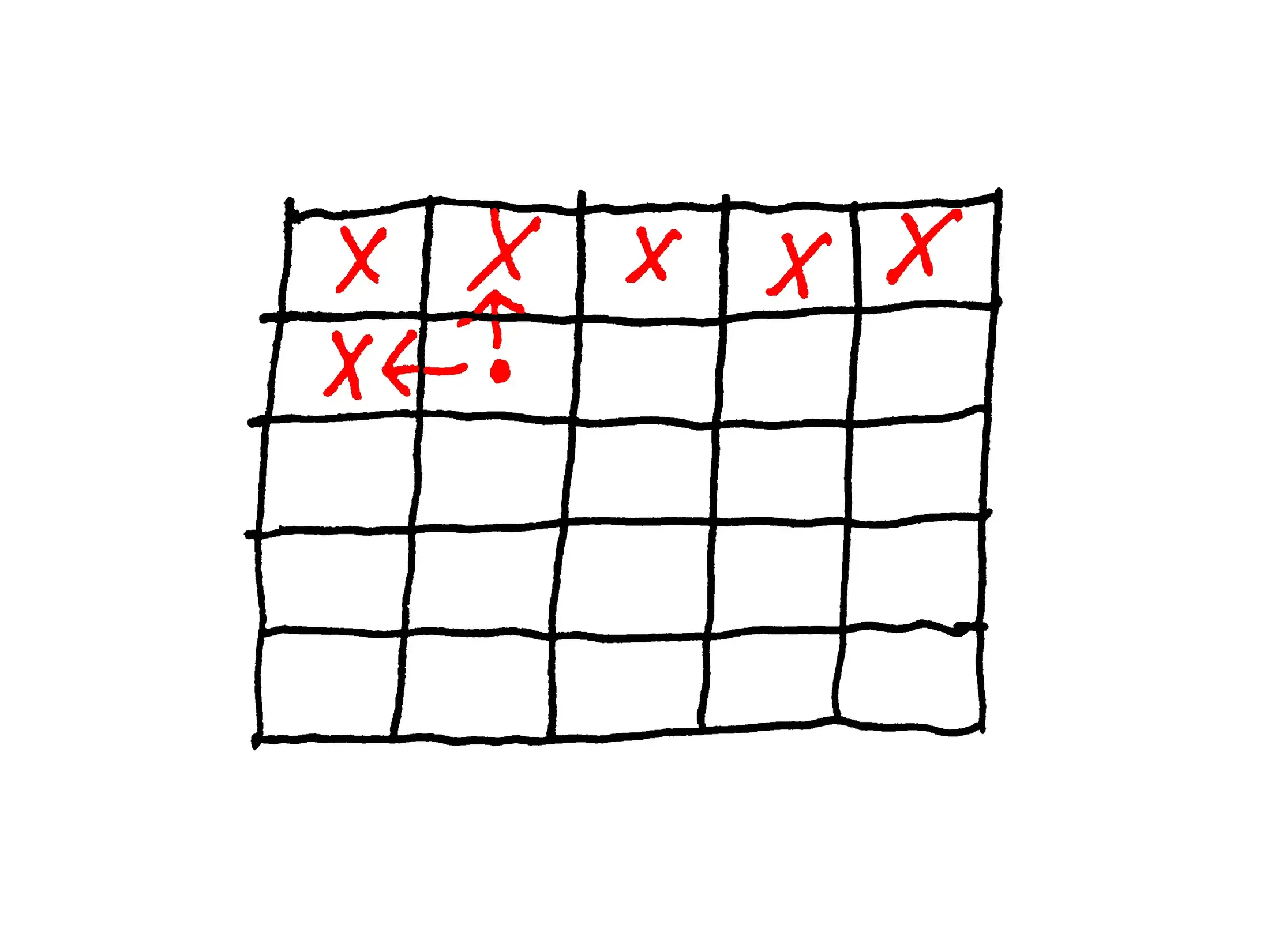
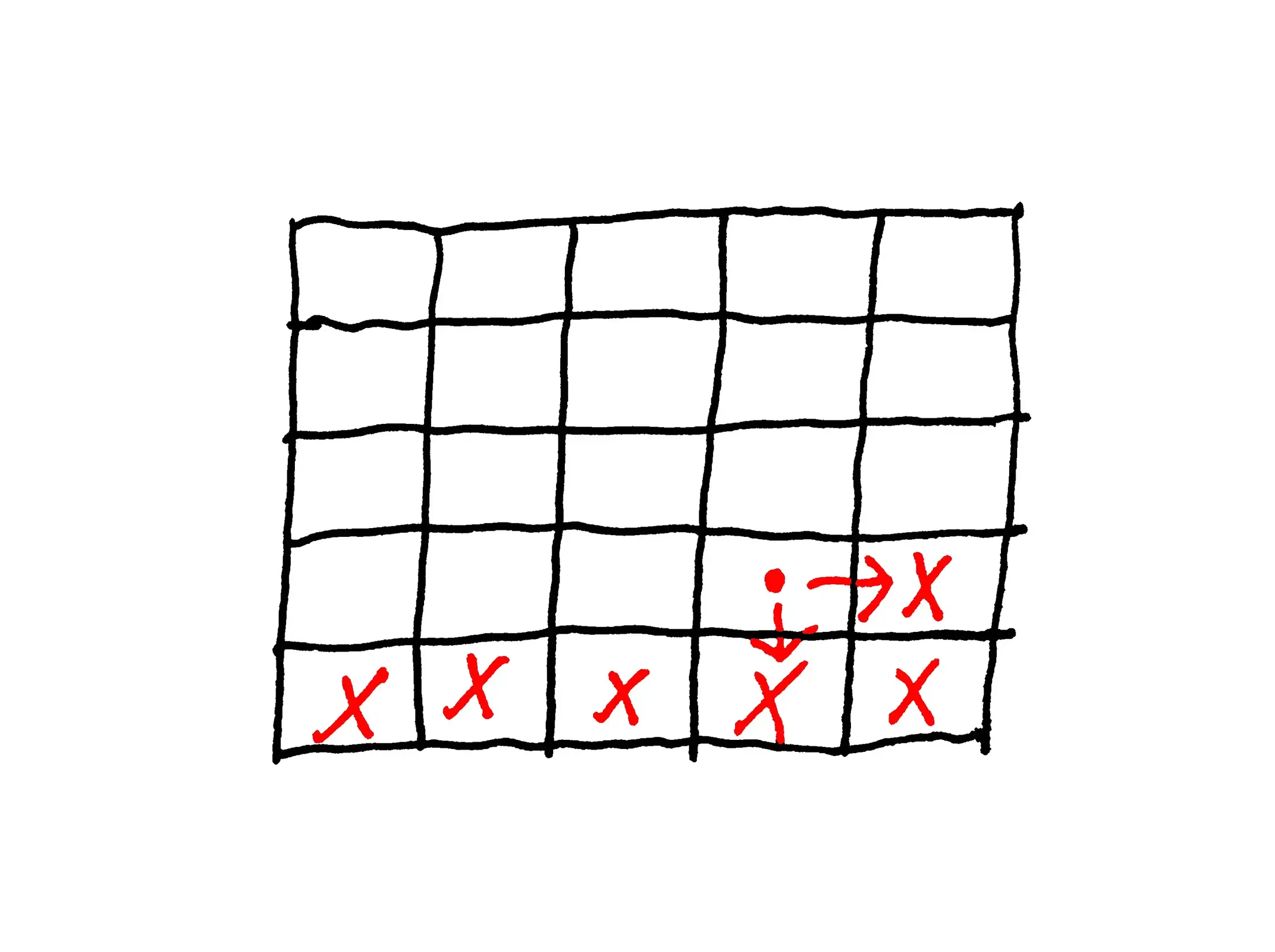
Propagation is the most important part of the whole algorithm; it's responsible for spreading the best matches to neighbors, acting kind of like a virus.
As mentioned previously, propagation and then random search are performed \(n\) times, which is important in propagation as its behavior changes every other iteration; when \(n\) is even you propagate forward, when \(n\) is odd you propagate in reverse.
In forward propagation you iterate over the image starting at the upper-left, moving right, row by row. For each pixel, you query the best match from the pixel to your left, comparing it to your best, if it's better you update your best. This process is then repeated with the pixel above you.
In reverse propagation you iterate over the image starting at the bottom-right, moving left, row by row. For each pixel, you query the best match from the pixel to your right, comparing it to your best, if it's better you update your best. This process is then repeated with the pixel below you.
The obvious question is why split up propagation into forward and reverse passes? You could simple iterate over the image once each pass, querying all cardinal neighbors.
Well on the forward pass, the left and top neighbors can continually spread a good match across the whole image. However, the right and bottom neighbors can't see the updated data, as you're scanning the image from left to right. This is why you need two passes, so the upper-left can spread to the bottom-right, and then the bottom-right can spread to the upper-left. You don't check all neighbors as it's a waste of time; two of the four neighbors can only see data from the previous iteration, not what's currently being updated.
Random Search
This is very straightforward, for each pixel you compute the offset to a random patch, then the best match is updated if the random one is better. This global random search has a search radius that shrinks each iteration until its minimum size is reached, initialized to half the image dimensions (it's a radius). The exact shrink schedule is up to you, but I've stuck with the schedule in the original paper; the search radius x and y are halved each iteration.
It should be noted that in the original paper this random search doesn't shrink between iterations. Instead each pixel does multiple random shrinking searches, until the search radius goes to 1; the search radius resets to max between pixels. Given the image pyramid strategy which will be explained later, this is unnecessary and significantly slows down the algorithm.
Convergence
The primary knobs which determine convergence are: PatchMatch iterations and random radius shrink schedule.
Typically, PatchMatch is just run for a fixed number of iterations (5-10) but I've also added an early convergence check; if between iterations less than 1% of the best matches improve, then it has converged.
I'll circle back and explain my iteration and shrink schedule after I introduce the image pyramid approach, as that changes the calculus.
Parallelizing PatchMatch (Wavefront)
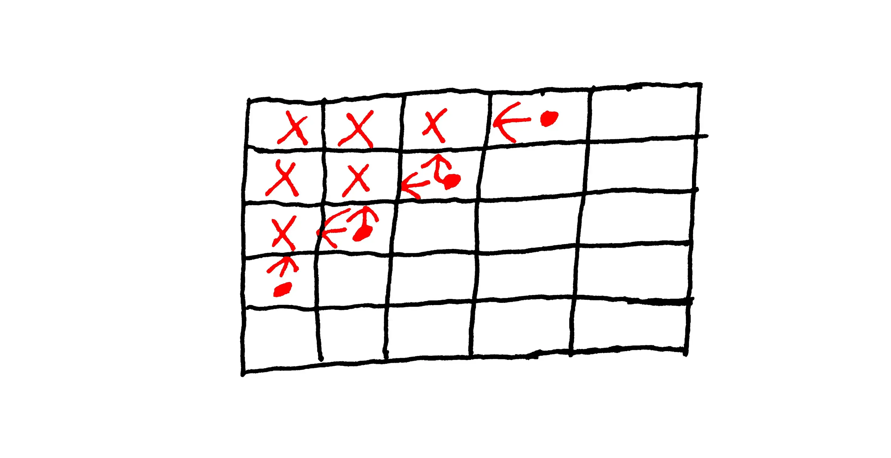
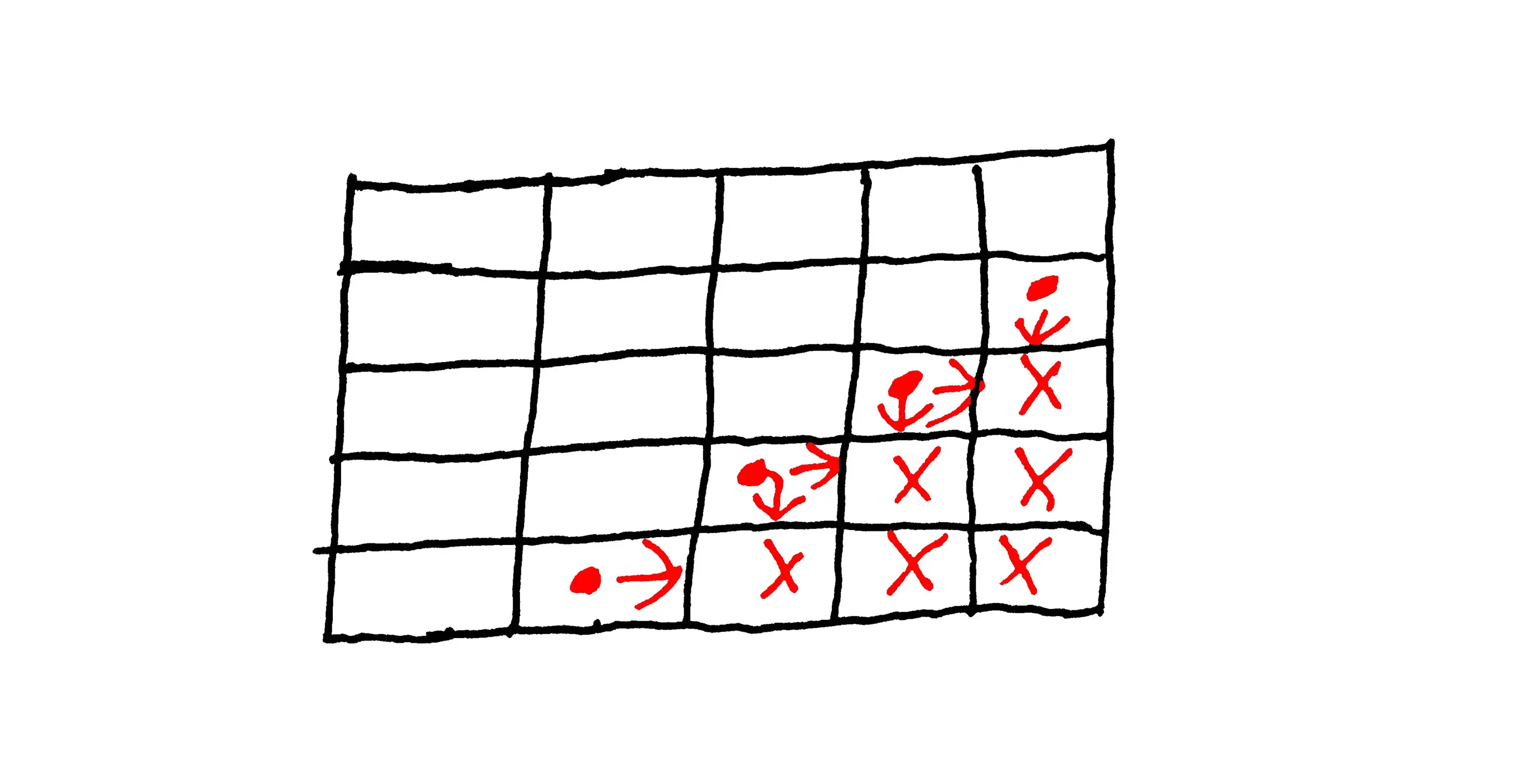
PatchMatch is not trivial to parallelize, as you can only look at neighbors which have been updated on the current scan. To solve this instead of iterating left to right in rows, you iterate over the anti-diagonals from upper-left to lower-right.
For example, when iterating over the forward pass anti-diagonals, the diagonal above will have been entirely updated already. This means you can independently split up the work of the current diagonal. Of course there are longer and shorter image diagonals, so most of the benefit is lost near the opposing image corners.
Modified PatchMatch (top-k)
With PatchMatch as I've described it, it will find the single most similar patch excluding the self-patch. This of course is insufficient for denoising, as we need to find the top-\(k\) matches. Only a small modification is needed for this change; instead of storing one match you store \(k\), and during propagation instead of comparing your best match to your neighbors best, you compare your worst match to your neighbors best; if your neighbors best match is better than your worst, you replace your worst.
There is another alternative where you propagate more than just the neighbors best match, but the best \(n\) of the top-\(k\). The idea is that given the patch regions are different, maybe your neighbors best match isn't better than your worst, but its second, or third, or fourth, etc, could be. However, it further complicates things by requiring more sorting, and I didn't find it very beneficial.
Picking K
The higher the \(k\) the higher the memory usage, but also the higher quality. Now the quality increase is true to a point, as picking too high of a \(k\) can actually cause over smoothing; \(k=40\) is the default as it's a good balance between memory usage and denoise quality. Below is a comparison of different \(k\) values:
For accurate comparison images are lossless; loading may be slow.

Image Pyramid
An image pyramid is a general image processing technique where you store multiple down/up scaled versions of your image, and do processing across scales. The processing starts from the largest/smallest resolution, and works up/down the pyramid; in this specific case \(n\) pyramid levels are created by halving the image resolution \(n-1\) times, processed from the lowest to highest image resolution. To be clear, the full PatchMatch algorithm is run at each image resolution. Now it may not be immediately apparent why you'd want to do this, as we want the algorithm to be fast, yet this requires doing more processing.
There are two entangled benefits of the image pyramid: it increase match quality while simultaneously decreasing computation time. This comes from doing more iterations on the lower resolution images where it's cheap, and doing less on the expensive high resolutions. Of course the algorithm speed is increased by doing cheaper iterations overall, but the higher quality comes from the global structure captured in the low resolutions; the low resolution levels provide approximate matching locations, which are further refined as the image resolution increases.
Importantly, for each pyramid level the error model must be recomputed, as noise statistics look different at the different resolutions. Similarly, the top-\(k\) similarity values must be recomputed when you jump to the next pyramid level, as otherwise they don't accurately reflect the similarity of previously found matches in the new level.
The image pyramid approach also changes how the random search should be approached; per-iteration random search not per-pixel is done because we can lean on the inherent global search in multi-scale processing. Furthermore, I found keeping the aggressive halving of the search radius to be beneficial; reducing the shrink rate causes more global matches to be found which are similar in noise statistics, but not in image content.
Denoising
The denoising calculations are essentially the same in KEEMY as in KEMY, except KEEMY doesn't have spatial distance weights; given the potential for global matches in KEEMY, a spatial weighting would negate that benefit. As such, denoising a pixel is simply the weighted average of patch centers, with a minimum weighting to the self-patch:
- Patch
- \(\text{Let } P \text{ be a Patch}\)
- Target Pixel
- \(\text{Let } t \text{ be the Target Pixel}\)
- Self-Patch Contribution
- \(\text{Let } w_{min} \text{ be the Self-Patch Contribution} \)
The above formula is for a single grayscale pixel, if it's a color image you simply do the same calculation per-channel.
However unlike KEMY, more than one denoise pass is typically required; the noisier the image the more passes required. Generally two passes is the sweet spot, but I don't recommend more than 5; doing more passes causes the noise to average out, but this can cause posterization; the range of colors decrease as pixel values converge to an average.
In addition to this, after every two passes the error model is rebuilt and the similarity scores are recomputed, using the current denoised image. I've found this to reduce some denoise artifacts, as the similarity values get stale when the underlying image content changes.
Below is a comparison of denoising a very noisy image at different pass levels:
For accurate comparison images are lossless; loading may be slow.

Optional Top-K Pruning
The similarity metric is incredibly discriminative, however it can still sometimes over smooth fine detail. An easy fix is to reduce the number of patches you're averaging over, but you're essentially just globally increasing the amount of noise. As such, a better method is to adaptively prune the number of matches you're averaging over.
There are many ways to prune the matches, but I went with a dynamic patch contribution method; after sorting the \(k\) candidate patches by similarity, they are accumulated into the final average only as long as they provide a significant update. Specifically, if a new patch’s weight represents less than some threshold like 1%, of the total weight accumulated so far the algorithm stops; this preserves detail by discarding low-similarity outliers while maintaining heavy smoothing in flat regions. With that being said, it can increase image noise if your threshold is too high, and importantly the threshold is relative so the effect changes with the number of \(k\).
For accurate comparison images are lossless; loading may be slow.
